Applying MCube to the 3D Drosophila embryo model
[1]:
set.seed(20240709)
library(MCube)
library(ggplot2)
[2]:
DATA_PATH <- "/import/home/share/zw/pql/data/Drosophila_embryo"
RESULT_PATH <- "/import/home/share/zw/pql/results/Drosophila_embryo"
if (!dir.exists(RESULT_PATH)) {
dir.create(RESULT_PATH, recursive = TRUE)
}
[3]:
n_slices <- 13
slice_idx_seq <- c(1:13)
reference_ST <- data.matrix(
read.csv(file.path(DATA_PATH, "reference_ST.csv"),
header = TRUE, row.names = 1, check.names = FALSE
)
)
dim(reference_ST)
num_celltypes <- nrow(reference_ST)
proportions_ST <- matrix(, nrow = 0, ncol = num_celltypes)
batch_id <- vector("character")
for (slice_idx in slice_idx_seq) {
proportions_i <- as.matrix(read.csv(
file.path(
DATA_PATH,
paste0("prop_slice", slice_idx - 1, ".csv")
),
header = TRUE, row.names = 1, check.names = FALSE
))
proportions_ST <- rbind(proportions_ST, proportions_i)
batch_id <- c(batch_id, rep(paste0("slice", slice_idx - 1), nrow(proportions_i)))
}
dim(proportions_ST)
num_spots <- nrow(proportions_ST)
spots <- rownames(proportions_ST)
names(batch_id) <- spots
counts <- as.data.frame(readr::read_csv(
file.path(DATA_PATH, "counts.csv")
))
rownames(counts) <- counts[, 1]
counts[, 1] <- NULL
counts <- counts[spots, ]
counts <- data.matrix(counts)
dim(counts)
coordinates <- data.matrix(read.csv(
file.path(DATA_PATH, "3D_coordinates.csv"),
header = TRUE, row.names = 1, check.names = FALSE
))
coordinates <- coordinates[spots, ]
dim(coordinates)
spot_effects_ST <- data.matrix(read.csv(
file.path(DATA_PATH, "spot_effects_ST.csv"),
header = TRUE, row.names = 1, check.names = FALSE
))[spots, 1]
platform_effects_ST <- data.matrix(read.csv(
file.path(DATA_PATH, "platform_effects_ST.csv"),
header = TRUE, row.names = 1, check.names = FALSE
))
library_sizes_ST <- data.matrix(read.csv(
file.path(DATA_PATH, "library_sizes_ST.csv"),
header = TRUE, row.names = 1, check.names = FALSE
))[spots, 1]
- 16
- 5838
- 14132
- 16
New names:
• `` -> `...1`
Rows: 14132 Columns: 5839
── Column specification ────────────────────────────────────────────────────────
Delimiter: ","
chr (1): ...1
dbl (5838): 14-3-3epsilon, 14-3-3zeta, 140up, 18SrRNA-Psi:CR41602, 26-29-p, ...
ℹ Use `spec()` to retrieve the full column specification for this data.
ℹ Specify the column types or set `show_col_types = FALSE` to quiet this message.
- 14132
- 5838
- 14132
- 3
Central nervous system
[4]:
celltype <- "CNS"
Correcting for slice-specific platform effects
[5]:
mcube_object <- createMCube(
counts = counts, coordinates = coordinates,
proportions = proportions_ST, library_sizes = library_sizes_ST,
covariates = NULL, batch_id = batch_id,
reference = reference_ST,
spot_effects = spot_effects_ST, platform_effects = platform_effects_ST,
celltype_test = celltype,
proportion_threshold = 0.5,
project = "CNS"
)
mcube_object <- mcubeFitNull(
mcube_object,
num_workers = 70, num_threads = 1
)
mcube_object <- mcubeTest(
mcube_object,
num_workers = 70, num_threads = 1, shared_memory = TRUE
)
Select high-abundance cell types to analyze with proportion_threshold = 0.5 and celltype_threshold = 100.
mcubeFilterCellTypes: Cell type(s) CNS, epidermis, fat body, foregut, midgut, muscle, salivary gland pass the threshold.
Cell type(s) CNS will be analyzed.
Filter out lowly-expressed genes with gene_threshold = 5e-05.
mcubeFilterGenes: 1482 genes pass the threshold.
Select highly-expressed genes to analyze for each specific cell type with reference_threshold = 0.5.
mcubeFilterGenesCellType: Select 392 genes to analyze for CNS.
Preprocessed data description: 14132 spots and 16 cell types in total. 546 spots, 392 genes, and 1 cell type(s) to analyze.
Number of physical cores: 72.
Number of workers: 70.
Number of thread(s) on BLAS per worker: 1.
mcubeKernel: length_scale is set as 0.178073578880044 for the Gaussian kernel.
mcubeKernel: length_scale is set as 0.251834070352474 for the Gaussian kernel.
mcubeKernel: length_scale is set as 0.178073578880044 for the Gaussian_transformed kernel.
mcubeKernel: length_scale is set as 0.251834070352474 for the Gaussian_transformed kernel.
Number of physical cores: 72.
Number of workers: 70.
Number of thread(s) on BLAS per worker: 1.
[6]:
saveRDS(
mcube_object,
file = file.path(
RESULT_PATH,
paste0("mcube_", celltype, ".rds")
)
)
# mcube_object <- readRDS(
# file = file.path(
# RESULT_PATH,
# paste0("mcube_", celltype, ".rds")
# )
# )
[7]:
nrow(mcube_object@pvalues[[1]])
sig_genes <- mcubeGetSigGenes(mcube_object@pvalues)
nrow(sig_genes[[1]])
head(sig_genes[[1]])
write.table(
rownames(sig_genes[[1]]),
file = file.path(
RESULT_PATH,
paste0("SVG_", celltype, ".txt")
),
quote = FALSE, row.names = FALSE, col.names = FALSE
)
346
mcubeGetSigGenes: Set adjust_method as BH and alpha as 0.05.
36
| pvalue | adjusted_pvalue | |
|---|---|---|
| <dbl> | <dbl> | |
| jim | 2.000158e-22 | 6.920548e-20 |
| fax | 2.059464e-13 | 3.562872e-11 |
| CG14989 | 4.907008e-11 | 5.659416e-09 |
| fabp | 1.365240e-10 | 1.180933e-08 |
| RpL39 | 2.037242e-08 | 1.409771e-06 |
| CG31323 | 4.807835e-07 | 2.772518e-05 |
[8]:
p <- mcubePlotPvalues(mcube_object@pvalues, "combined_pvalue") +
xlim(c(0, 4)) +
ggtitle("CNS") +
coord_fixed(ratio = 1) +
theme(
plot.title = element_text(size = 24),
axis.title.x = element_text(size = 24),
axis.title.y = element_text(size = 24),
axis.text.x = element_text(size = 16),
axis.text.y = element_text(size = 16),
legend.position = "none"
)
ggsave(
file = file.path(RESULT_PATH, paste0(celltype, "_combined_pvalue.pdf")),
plot = p, width = 5, height = 5
)
p
Coordinate system already present. Adding new coordinate system, which will
replace the existing one.

[9]:
# # For saving the plotly object as a static image with `kaleido`
# install.packages('reticulate')
# reticulate::install_miniconda()
# reticulate::conda_install('r-reticulate', 'python-kaleido')
# reticulate::conda_install('r-reticulate', 'plotly', channel = 'plotly')
# reticulate::use_miniconda('r-reticulate')
[10]:
# Proportions in the 3D perspective
p <- mcubePlotPropCellType3D(
mcube_object@proportions, mcube_object@coordinates, celltype, proportion_threshold = 0.5,
spot_size = 1.5, opacity_target = 0.8, opacity_background = 0.05,
axis_rescale = c(1, 1, 1.5), plotly_eye = list(x = 0.2, y = -1.5, z = 1.6)
)
plotly::save_image(
p, file.path(RESULT_PATH, paste0("proportion_", celltype, "_3D", ".pdf")),
width = 600, height = 400, scale = 5
)
p
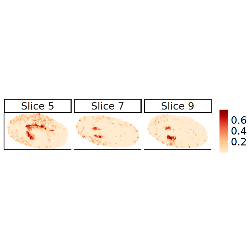
[11]:
# Proportions in the 2D perspective
slices_plot <- c(5, 7, 9)
spots_plot <- rownames(mcube_object@proportions)[
mcube_object@batch_id %in% paste0("slice", slices_plot - 1)
]
proportions_long <- data.frame(
mcube_object@coordinates[spots_plot, c("x", "y")],
proportion = mcube_object@proportions[spots_plot, celltype],
slice = paste(
"Slice",
as.integer(gsub("slice([0-9]+)", "\\1", mcube_object@batch_id[spots_plot])) + 1
)
)
# head(proportions_long)
[12]:
p <- ggplot(proportions_long, aes(x = x, y = y)) +
geom_point(aes(color = proportion), size = 1, alpha = 1) +
scale_colour_gradientn(name = NULL, colors = pals::brewer.orrd(22)[3:22]) +
coord_fixed(ratio = 1) +
facet_wrap(. ~ slice, nrow = 1) +
labs(
title = "Estimated cell type proportions by STitch3D",
x = "x", y = "y"
) +
theme_classic() +
theme(
text = element_text(family = "Helvetica"),
plot.title = element_blank(),
axis.text = element_blank(),
axis.ticks = element_blank(),
axis.title.x = element_blank(),
axis.title.y = element_blank(),
strip.text = element_text(size = 20),
legend.title = element_blank(),
legend.text = element_text(size = 20),
legend.position = "right"
)
ggsave(
filename = file.path(
RESULT_PATH, paste0("proportion_", celltype, ".pdf")
),
plot = p, width = 12, height = 3
)
ggsave(
filename = file.path(
RESULT_PATH, paste0("proportion_", celltype, ".png")
),
plot = p, width = 12, height = 3
)
p
[13]:
demo_genes <- c("jim", "fax", "CG14989", "fabp", "14-3-3epsilon")
mcube_object@pvalues[[1]][demo_genes, ]
for (gene in demo_genes) {
p <- mcubePlotExprCellType3D(
object = mcube_object, gene = gene, celltype = celltype, proportion_threshold = 0.5,
spot_size = 1.5, opacity_target = 0.8, opacity_background = 0.05,
axis_rescale = c(1, 1, 1.5), plotly_eye = list(x = 0.2, y = -1.5, z = 1.6)
)
plotly::save_image(
p, file.path(RESULT_PATH, paste0(celltype, "_", gene, ".pdf")),
width = 600, height = 400, scale = 5
)
}
p
| linear | Gaussian_1 | Gaussian_2 | Gaussian_transformed_1 | Gaussian_transformed_2 | combined_pvalue | |
|---|---|---|---|---|---|---|
| <dbl> | <dbl> | <dbl> | <dbl> | <dbl> | <dbl> | |
| jim | 2.483974e-04 | 2.000158e-22 | 1.391063e-20 | 2.411920e-06 | 3.517968e-06 | 2.000158e-22 |
| fax | 1.331406e-13 | 9.864353e-13 | 6.344871e-14 | 7.131344e-07 | 1.178233e-07 | 2.059464e-13 |
| CG14989 | 7.349526e-08 | 1.356572e-11 | 3.550379e-11 | 8.367655e-05 | 1.541567e-05 | 4.907008e-11 |
| fabp | 1.500675e-07 | 7.013068e-10 | 2.841780e-11 | 3.329066e-06 | 6.366401e-07 | 1.365240e-10 |
| 14-3-3epsilon | 1.147463e-06 | 4.298401e-05 | 2.535075e-05 | 1.513034e-04 | 4.390764e-05 | 5.188966e-06 |
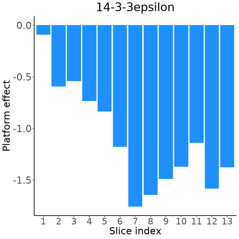
[14]:
# Visualizing the slice-specific platform effects
slice_idx_seq_plot <- factor(slice_idx_seq, levels = slice_idx_seq)
for (gene in demo_genes) {
p <- ggplot(data = NULL, aes(x = slice_idx_seq_plot, y = platform_effects_ST[, gene])) +
geom_bar(stat = "identity", fill = "dodgerblue") +
labs(title = gene, x = "Slice index", y = "Platform effect") +
theme_classic() +
theme(
text = element_text(family = "Helvetica", size = 20),
plot.title = element_text(size = 24, hjust = 0.5, face = "italic"),
axis.title = element_text(size = 20),
axis.text.x = element_text(size = 18),
axis.text.y = element_text(size = 20)
)
ggsave(
filename = file.path(
RESULT_PATH,
paste0(
"platform_effects_", gene,
".pdf"
)
),
plot = p, width = 5, height = 4
)
}
p
Not considering slice-specific platform effects
[15]:
mcube_object_batch_effects <- createMCube(
counts = counts, coordinates = coordinates,
proportions = proportions_ST, library_sizes = library_sizes_ST,
covariates = NULL, batch_id = NULL, # Assume all spots from the same batch by setting batch_id as NULL
reference = reference_ST,
spot_effects = spot_effects_ST, platform_effects = NULL,
celltype_test = celltype,
proportion_threshold = 0.5,
project = "CNS"
)
mcube_object_batch_effects <- mcubeFitNull(
mcube_object_batch_effects,
num_workers = 70, num_threads = 1
)
mcube_object_batch_effects <- mcubeTest(
mcube_object_batch_effects,
num_workers = 70, num_threads = 1, shared_memory = TRUE
)
saveRDS(
mcube_object_batch_effects,
file = file.path(
RESULT_PATH,
paste0(
"mcube_", celltype,
"_batch_effects",
".rds"
)
)
)
The batch_id is not provided!
All spots are assumed to be from the same batch and share the same gene platform effects.
Select high-abundance cell types to analyze with proportion_threshold = 0.5 and celltype_threshold = 100.
mcubeFilterCellTypes: Cell type(s) CNS, epidermis, fat body, foregut, midgut, muscle, salivary gland pass the threshold.
Cell type(s) CNS will be analyzed.
Filter out lowly-expressed genes with gene_threshold = 5e-05.
mcubeFilterGenes: 1482 genes pass the threshold.
The platform effects are not provided and need to be estimated from data!
Select highly-expressed genes to analyze for each specific cell type with reference_threshold = 0.5.
mcubeFilterGenesCellType: Select 392 genes to analyze for CNS.
Preprocessed data description: 14132 spots and 16 cell types in total. 546 spots, 392 genes, and 1 cell type(s) to analyze.
Number of physical cores: 72.
Number of workers: 70.
Number of thread(s) on BLAS per worker: 1.
mcubeKernel: length_scale is set as 0.178073578880044 for the Gaussian kernel.
mcubeKernel: length_scale is set as 0.251834070352474 for the Gaussian kernel.
mcubeKernel: length_scale is set as 0.178073578880044 for the Gaussian_transformed kernel.
mcubeKernel: length_scale is set as 0.251834070352474 for the Gaussian_transformed kernel.
Number of physical cores: 72.
Number of workers: 70.
Number of thread(s) on BLAS per worker: 1.
[16]:
nrow(mcube_object_batch_effects@pvalues[[1]])
sig_genes <- mcubeGetSigGenes(mcube_object_batch_effects@pvalues)
nrow(sig_genes[[1]])
head(sig_genes[[1]])
346
mcubeGetSigGenes: Set adjust_method as BH and alpha as 0.05.
44
| pvalue | adjusted_pvalue | |
|---|---|---|
| <dbl> | <dbl> | |
| jim | 7.340192e-27 | 2.539706e-24 |
| Atpalpha | 1.643130e-14 | 2.842615e-12 |
| mt:ATPase6 | 1.152411e-12 | 1.265060e-10 |
| RpL39 | 1.462497e-12 | 1.265060e-10 |
| CG14989 | 4.188065e-10 | 2.898141e-08 |
| Vmat | 1.972257e-08 | 1.137335e-06 |
Salivary gland
[17]:
celltype <- "salivary gland"
spots_names <- rownames(proportions_ST)[proportions_ST[, celltype] > 0.5]
Correcting for slice-specific platform effects
[18]:
mcube_object <- createMCube(
counts = counts, coordinates = coordinates,
proportions = proportions_ST, library_sizes = library_sizes_ST,
covariates = NULL, batch_id = batch_id,
reference = reference_ST,
spot_effects = spot_effects_ST, platform_effects = platform_effects_ST,
celltype_test = celltype,
proportion_threshold = 0.5,
project = "salivary gland"
)
mcube_object <- mcubeFitNull(
mcube_object,
num_workers = 70, num_threads = 1
)
mcube_object <- mcubeTest(
mcube_object,
num_workers = 70, num_threads = 1, shared_memory = TRUE
)
Select high-abundance cell types to analyze with proportion_threshold = 0.5 and celltype_threshold = 100.
mcubeFilterCellTypes: Cell type(s) CNS, epidermis, fat body, foregut, midgut, muscle, salivary gland pass the threshold.
Cell type(s) salivary gland will be analyzed.
Filter out lowly-expressed genes with gene_threshold = 5e-05.
mcubeFilterGenes: 1482 genes pass the threshold.
Select highly-expressed genes to analyze for each specific cell type with reference_threshold = 0.5.
mcubeFilterGenesCellType: Select 619 genes to analyze for salivary gland.
Preprocessed data description: 14132 spots and 16 cell types in total. 176 spots, 619 genes, and 1 cell type(s) to analyze.
Number of physical cores: 72.
Number of workers: 70.
Number of thread(s) on BLAS per worker: 1.
mcubeKernel: length_scale is set as 0.178073578880044 for the Gaussian kernel.
mcubeKernel: length_scale is set as 0.251834070352474 for the Gaussian kernel.
mcubeKernel: length_scale is set as 0.178073578880044 for the Gaussian_transformed kernel.
mcubeKernel: length_scale is set as 0.251834070352474 for the Gaussian_transformed kernel.
Number of physical cores: 72.
Number of workers: 70.
Number of thread(s) on BLAS per worker: 1.
[19]:
saveRDS(
mcube_object,
file = file.path(
RESULT_PATH,
paste0("mcube_", "salivary_gland", ".rds")
)
)
# mcube_object <- readRDS(
# file = file.path(
# RESULT_PATH,
# paste0("mcube_", "salivary_gland", ".rds")
# )
# )
[20]:
nrow(mcube_object@pvalues[[1]])
sig_genes <- mcubeGetSigGenes(mcube_object@pvalues)
nrow(sig_genes[[1]])
head(sig_genes[[1]])
write.table(
rownames(sig_genes[[1]]),
file = file.path(
RESULT_PATH,
paste0("SVG_", "salivary_gland", ".txt")
),
quote = FALSE, row.names = FALSE, col.names = FALSE
)
553
mcubeGetSigGenes: Set adjust_method as BH and alpha as 0.05.
9
| pvalue | adjusted_pvalue | |
|---|---|---|
| <dbl> | <dbl> | |
| CG13159 | 1.243477e-18 | 6.876427e-16 |
| CG43181 | 2.555733e-13 | 5.783440e-11 |
| nur | 3.137490e-13 | 5.783440e-11 |
| PPO1 | 1.749047e-07 | 2.418058e-05 |
| CG14265 | 4.323899e-06 | 4.782232e-04 |
| CG14636 | 1.279481e-05 | 1.179255e-03 |
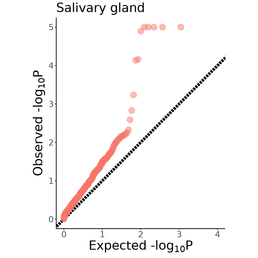
[21]:
p <- mcubePlotPvalues(mcube_object@pvalues, "combined_pvalue") +
xlim(c(0, 4)) +
ggtitle("Salivary gland") +
coord_fixed(ratio = 1) +
theme(
plot.title = element_text(size = 24),
axis.title.x = element_text(size = 24),
axis.title.y = element_text(size = 24),
axis.text.x = element_text(size = 16),
axis.text.y = element_text(size = 16),
legend.position = "none"
)
ggsave(
file = file.path(RESULT_PATH, paste0("salivary_gland", "_combined_pvalue.pdf")),
plot = p, width = 5, height = 5
)
p
Coordinate system already present. Adding new coordinate system, which will
replace the existing one.
[22]:
# Proportions in the 3D perspective
p <- mcubePlotPropCellType3D(
mcube_object@proportions, mcube_object@coordinates, celltype, proportion_threshold = 0.5,
spot_size = 1.5, opacity_target = 0.8, opacity_background = 0.05,
axis_rescale = c(1, 1, 1.5), plotly_eye = list(x = -0.1, y = -1.6, z = 1.8)
)
plotly::save_image(
p, file.path(RESULT_PATH, paste0("proportion_", "salivary_gland", "_3D", ".pdf")),
width = 600, height = 400, scale = 5
)
p
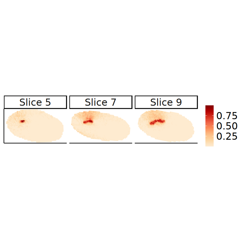
[23]:
slices_plot <- c(5, 7, 9)
spots_plot <- rownames(mcube_object@proportions)[
mcube_object@batch_id %in% paste0("slice", slices_plot - 1)
]
proportions_long <- data.frame(
mcube_object@coordinates[spots_plot, c("x", "y")],
proportion = mcube_object@proportions[spots_plot, celltype],
slice = paste(
"Slice",
as.integer(gsub("slice([0-9]+)", "\\1", mcube_object@batch_id[spots_plot])) + 1
)
)
# head(proportions_long)
[24]:
# Proportions in the 2D perspective
p <- ggplot(proportions_long, aes(x = x, y = y)) +
geom_point(aes(color = proportion), size = 1, alpha = 1) +
scale_colour_gradientn(name = NULL, colors = pals::brewer.orrd(22)[3:22]) +
coord_fixed(ratio = 1) +
facet_wrap(. ~ slice, nrow = 1) +
labs(
title = "Estimated cell type proportions by STitch3D",
x = "x", y = "y"
) +
theme_classic() +
theme(
text = element_text(family = "Helvetica"),
plot.title = element_blank(),
axis.text = element_blank(),
axis.ticks = element_blank(),
axis.title.x = element_blank(),
axis.title.y = element_blank(),
strip.text = element_text(size = 20),
legend.title = element_blank(),
legend.text = element_text(size = 20),
legend.position = "right"
)
ggsave(
filename = file.path(
RESULT_PATH, paste0("proportion_", celltype, ".pdf")
),
plot = p, width = 12, height = 3
)
ggsave(
filename = file.path(
RESULT_PATH, paste0("proportion_", celltype, ".png")
),
plot = p, width = 12, height = 3
)
p
[25]:
demo_genes <- c("CG13159", "CG43181", "nur", "PPO1", "CG14265")
mcube_object@pvalues[[1]][demo_genes, ]
for (gene in demo_genes) {
p <- mcubePlotExprCellType3D(
object = mcube_object, gene = gene, celltype = celltype, proportion_threshold = 0.5,
spot_size = 1.5, opacity_target = 0.8, opacity_background = 0.05,
plotly_eye = list(x = -0.1, y = -1.6, z = 1.8)
)
plotly::save_image(
p, file.path(RESULT_PATH, paste0("salivary_gland", "_", gene, ".pdf")),
width = 600, height = 400, scale = 5
)
}
p
| linear | Gaussian_1 | Gaussian_2 | Gaussian_transformed_1 | Gaussian_transformed_2 | combined_pvalue | |
|---|---|---|---|---|---|---|
| <dbl> | <dbl> | <dbl> | <dbl> | <dbl> | <dbl> | |
| CG13159 | 3.976520e-12 | 1.243477e-18 | 6.249950e-18 | 1.318915e-11 | 6.884301e-12 | 1.243477e-18 |
| CG43181 | 2.832925e-02 | 5.275890e-14 | 1.646601e-12 | 3.454043e-05 | 7.333662e-08 | 2.555733e-13 |
| nur | 2.313631e-08 | 6.775868e-14 | 8.414646e-13 | 1.540838e-09 | 4.672384e-09 | 3.137490e-13 |
| PPO1 | 5.807640e-03 | 3.834335e-08 | 4.000800e-07 | 2.329759e-03 | 1.481691e-04 | 1.749047e-07 |
| CG14265 | 1.597989e-01 | 1.709103e-06 | 1.845853e-06 | 7.348261e-04 | 3.553659e-05 | 4.323899e-06 |
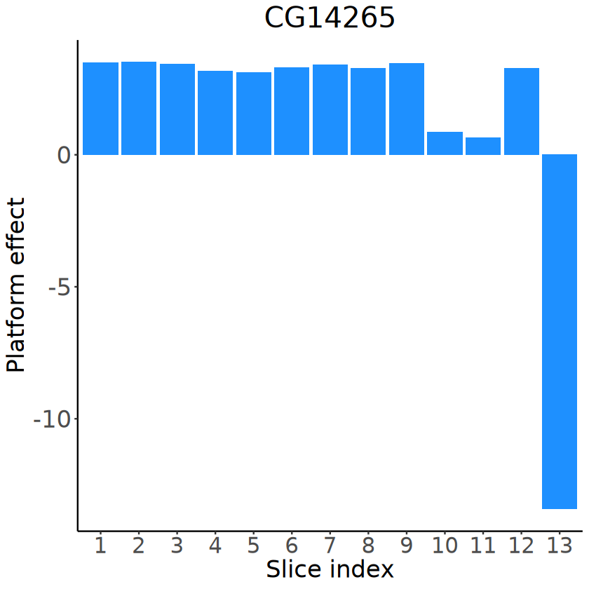
[26]:
# Visualizing the slice-specific platform effects
slice_idx_seq_plot <- factor(slice_idx_seq, levels = slice_idx_seq)
for (gene in demo_genes) {
p <- ggplot(data = NULL, aes(x = slice_idx_seq_plot, y = platform_effects_ST[, gene])) +
geom_bar(stat = "identity", fill = "dodgerblue") +
labs(title = gene, x = "Slice index", y = "Platform effect") +
theme_classic() +
theme(
text = element_text(family = "Helvetica", size = 20),
plot.title = element_text(size = 24, hjust = 0.5, face = "italic"),
axis.title = element_text(size = 20),
axis.text.x = element_text(size = 18),
axis.text.y = element_text(size = 20)
)
ggsave(
filename = file.path(
RESULT_PATH,
paste0(
"platform_effects_", gene,
".pdf"
)
),
plot = p, width = 5, height = 4
)
}
p
Not considering slice-specific platform effects
[27]:
mcube_object_batch_effects <- createMCube(
counts = counts, coordinates = coordinates,
proportions = proportions_ST, library_sizes = library_sizes_ST,
covariates = NULL, batch_id = NULL, # Assume all spots from the same batch by setting batch_id as NULL
reference = reference_ST,
spot_effects = spot_effects_ST, platform_effects = NULL,
celltype_test = celltype,
proportion_threshold = 0.5,
project = "salivary gland"
)
mcube_object_batch_effects <- mcubeFitNull(
mcube_object_batch_effects,
num_workers = 70, num_threads = 1
)
mcube_object_batch_effects <- mcubeTest(
mcube_object_batch_effects,
num_workers = 70, num_threads = 1, shared_memory = TRUE
)
saveRDS(
mcube_object_batch_effects,
file = file.path(
RESULT_PATH,
paste0(
"mcube_", "salivary_gland",
"_batch_effects",
".rds"
)
)
)
The batch_id is not provided!
All spots are assumed to be from the same batch and share the same gene platform effects.
Select high-abundance cell types to analyze with proportion_threshold = 0.5 and celltype_threshold = 100.
mcubeFilterCellTypes: Cell type(s) CNS, epidermis, fat body, foregut, midgut, muscle, salivary gland pass the threshold.
Cell type(s) salivary gland will be analyzed.
Filter out lowly-expressed genes with gene_threshold = 5e-05.
mcubeFilterGenes: 1482 genes pass the threshold.
The platform effects are not provided and need to be estimated from data!
Select highly-expressed genes to analyze for each specific cell type with reference_threshold = 0.5.
mcubeFilterGenesCellType: Select 619 genes to analyze for salivary gland.
Preprocessed data description: 14132 spots and 16 cell types in total. 176 spots, 619 genes, and 1 cell type(s) to analyze.
Number of physical cores: 72.
Number of workers: 70.
Number of thread(s) on BLAS per worker: 1.
mcubeKernel: length_scale is set as 0.178073578880044 for the Gaussian kernel.
mcubeKernel: length_scale is set as 0.251834070352474 for the Gaussian kernel.
mcubeKernel: length_scale is set as 0.178073578880044 for the Gaussian_transformed kernel.
mcubeKernel: length_scale is set as 0.251834070352474 for the Gaussian_transformed kernel.
Number of physical cores: 72.
Number of workers: 70.
Number of thread(s) on BLAS per worker: 1.
[28]:
nrow(mcube_object_batch_effects@pvalues[[1]])
sig_genes <- mcubeGetSigGenes(mcube_object_batch_effects@pvalues)
nrow(sig_genes[[1]])
head(sig_genes[[1]])
553
mcubeGetSigGenes: Set adjust_method as BH and alpha as 0.05.
30
| pvalue | adjusted_pvalue | |
|---|---|---|
| <dbl> | <dbl> | |
| CG13159 | 4.424356e-23 | 2.446669e-20 |
| nur | 1.199964e-18 | 3.317900e-16 |
| CG18649 | 1.953955e-18 | 3.601791e-16 |
| CG43181 | 5.717649e-14 | 7.904649e-12 |
| CG13738 | 4.927461e-10 | 5.449771e-08 |
| CG32453 | 8.905072e-10 | 8.207508e-08 |
[ ]: