Applying MCube to the DLPFC dataset
[1]:
set.seed(20240709)
library(MCube)
library(ggplot2)
[2]:
RAW_DATA_PATH <- "/import/home/share/zw/data/DLPFC" # H&E images
DATA_PATH <- "/import/home/share/zw/pql/data/DLPFC"
RESULT_PATH <- "/import/home/share/zw/pql/results/DLPFC"

if (!dir.exists(file.path(RESULT_PATH))) {
    dir.create(file.path(RESULT_PATH), recursive = TRUE)
}
[3]:
# Load in data and cell type deconvolution results

n_slices <- 4
slice_idx_seq <- c(151673, 151674, 151675, 151676)

reference_ST <- data.matrix(
    read.csv(file.path(DATA_PATH, "reference_ST.csv"),
        header = TRUE, row.names = 1, check.names = FALSE
    )
)
dim(reference_ST)
num_celltypes <- nrow(reference_ST)

proportions_ST <- matrix(, nrow = 0, ncol = num_celltypes)
batch_id <- vector("character")
for(i in 1:n_slices){
    proportions_i <- as.matrix(read.csv(
        file.path(
            DATA_PATH,
            paste0("prop_slice", i - 1, ".csv")
        ),
        header = TRUE, row.names = 1, check.names = FALSE
    ))
    proportions_ST <- rbind(proportions_ST, proportions_i)
    batch_id <- c(batch_id, rep(paste0("slice_", slice_idx_seq[i]), nrow(proportions_i)))
}
dim(proportions_ST)
num_spots <- nrow(proportions_ST)
spots <- rownames(proportions_ST)
names(batch_id) <- spots


counts <- as.data.frame(readr::read_csv(
    file.path(DATA_PATH, "counts.csv")
))
rownames(counts) <- counts[, 1]
counts[, 1] <- NULL
counts <- counts[spots, ]
counts <- data.matrix(counts)
dim(counts)

coordinates <- as.matrix(read.csv(
    file.path(DATA_PATH, "3D_coordinates.csv"),
    header = TRUE, row.names = 1, check.names = FALSE
))
coordinates <- coordinates[spots, ]
dim(coordinates)

spot_effects_ST <- data.matrix(read.csv(
    file.path(DATA_PATH, "spot_effects_ST.csv"),
    header = TRUE, row.names = 1, check.names = FALSE
))[spots, 1]

platform_effects_ST <- data.matrix(read.csv(
    file.path(DATA_PATH, "platform_effects_ST.csv"),
    header = TRUE, row.names = 1, check.names = FALSE
))
rownames(platform_effects_ST) <- paste0("slice_", slice_idx_seq)

library_sizes_ST <- data.matrix(read.csv(
    file.path(DATA_PATH, "library_sizes_ST.csv"),
    header = TRUE, row.names = 1, check.names = FALSE
))[spots, 1]
- 18
- 4558
- 14243
- 18
New names:
• `` -> `...1`
Rows: 14243 Columns: 4559
── Column specification ────────────────────────────────────────────────────────
Delimiter: ","
chr    (1): ...1
dbl (4558): A2M, AAK1, AASDHPPT, AASS, AATK, ABCA1, ABCA2, ABCA5, ABCA8, ABC...

ℹ Use `spec()` to retrieve the full column specification for this data.
ℹ Specify the column types or set `show_col_types = FALSE` to quiet this message.
- 14243
- 4558
- 14243
- 3
Applying MCube to each ST slice seperately
[4]:
for (slice_idx in slice_idx_seq) {
    spots_used <- which(batch_id == paste0("slice_", slice_idx))
    mcube_object <- createMCube(
        counts = counts[spots_used, ],
        coordinates = coordinates[spots_used, c("x", "y")],
        proportions = proportions_ST[spots_used, ],
        library_sizes = library_sizes_ST[spots_used],
        covariates = NULL, batch_id = batch_id[spots_used],
        reference = reference_ST,
        spot_effects = spot_effects_ST[spots_used],
        platform_effects = NULL, # Estimate platform effects automatically in the single slice case
        reference_threshold = 0.5,
        project = paste0("DLPFC_", slice_idx),
    )
    mcube_object <- mcubeFitNull(
        mcube_object,
        num_workers = 70, num_threads = 1
    )
    mcube_object <- mcubeTest(
        mcube_object,
        num_workers = 70, num_threads = 1,
        shared_memory = TRUE
    )

    p <- mcubePlotPvalues(mcube_object@pvalues, "combined_pvalue", nrow = 2)
    p <- p +
        labs(title = NULL) +
        theme(
            text = element_text(size = 16),
            plot.title = element_text(size = 20),
            axis.title = element_text(size = 20),
            axis.text.x = element_text(size = 16),
            axis.text.y = element_text(size = 16)
        )
    ggsave(
        filename = file.path(
            RESULT_PATH,
            paste0("pvalue_qqplot_", slice_idx, ".png")
        ),
        plot = p, width = 12, height = 7
    )

    saveRDS(
        mcube_object,
        file = file.path(
            RESULT_PATH,
            paste0("mcube_", slice_idx, ".rds")
        )
    )
    assign(
        paste0("mcube_object_", slice_idx),
        mcube_object
    )
    rm(mcube_object)
}
Select high-abundance cell types to analyze with proportion_threshold = 0.1 and celltype_threshold = 100.

mcubeFilterCellTypes: Cell type(s) Astros_3, Ex_10_L2_4, Ex_2_L5, Ex_5_L5, Ex_7_L4_6, Ex_8_L5_6, Oligos_1, Oligos_3 pass the threshold.

Cell type(s) Astros_1, Astros_2, Endo, Ex_1_L5_6, Ex_3_L4_5, Ex_4_L_6, Ex_6_L4_6, Ex_9_L5_6, Micro/Macro, Oligos_2 has/have less than the minimum celltype_threshold = 100 with proportion_threshold = 0.1.
To include the above cell type(s), please reduce celltype_threshold or proportion_threshold.

Cell type(s) Astros_3, Ex_10_L2_4, Ex_2_L5, Ex_5_L5, Ex_7_L4_6, Ex_8_L5_6, Oligos_1, Oligos_3 will be analyzed.

Filter out lowly-expressed genes with gene_threshold = 5e-05.

mcubeFilterGenes: 2193 genes pass the threshold.

The platform effects are not provided and need to be estimated from data!

Select highly-expressed genes to analyze for each specific cell type with reference_threshold = 0.5.

mcubeFilterGenesCellType: Select 775 genes to analyze for Astros_3.

mcubeFilterGenesCellType: Select 709 genes to analyze for Ex_10_L2_4.

mcubeFilterGenesCellType: Select 1049 genes to analyze for Ex_2_L5.

mcubeFilterGenesCellType: Select 1112 genes to analyze for Ex_5_L5.

mcubeFilterGenesCellType: Select 696 genes to analyze for Ex_7_L4_6.

mcubeFilterGenesCellType: Select 691 genes to analyze for Ex_8_L5_6.

mcubeFilterGenesCellType: Select 780 genes to analyze for Oligos_1.

mcubeFilterGenesCellType: Select 773 genes to analyze for Oligos_3.

Preprocessed data description: 3611 spots and 18 cell types in total. 3606 spots, 2180 genes, and 8 cell type(s) to analyze.

Number of physical cores: 72.

Number of workers: 70.

Number of thread(s) on BLAS per worker: 1.

mcubeKernel: length_scale is set as 0.10891969400686 for the Gaussian kernel.

mcubeKernel: length_scale is set as 0.154035708474029 for the Gaussian kernel.

mcubeKernel: length_scale is set as 0.10891969400686 for the Gaussian_transformed kernel.

mcubeKernel: length_scale is set as 0.154035708474029 for the Gaussian_transformed kernel.

Number of physical cores: 72.

Number of workers: 70.

Number of thread(s) on BLAS per worker: 1.

Select high-abundance cell types to analyze with proportion_threshold = 0.1 and celltype_threshold = 100.

mcubeFilterCellTypes: Cell type(s) Astros_3, Ex_10_L2_4, Ex_5_L5, Ex_7_L4_6, Ex_8_L5_6, Oligos_1, Oligos_3 pass the threshold.

Cell type(s) Astros_1, Astros_2, Endo, Ex_1_L5_6, Ex_2_L5, Ex_3_L4_5, Ex_4_L_6, Ex_6_L4_6, Ex_9_L5_6, Micro/Macro, Oligos_2 has/have less than the minimum celltype_threshold = 100 with proportion_threshold = 0.1.
To include the above cell type(s), please reduce celltype_threshold or proportion_threshold.

Cell type(s) Astros_3, Ex_10_L2_4, Ex_5_L5, Ex_7_L4_6, Ex_8_L5_6, Oligos_1, Oligos_3 will be analyzed.

Filter out lowly-expressed genes with gene_threshold = 5e-05.

mcubeFilterGenes: 2230 genes pass the threshold.

The platform effects are not provided and need to be estimated from data!

Select highly-expressed genes to analyze for each specific cell type with reference_threshold = 0.5.

mcubeFilterGenesCellType: Select 822 genes to analyze for Astros_3.

mcubeFilterGenesCellType: Select 741 genes to analyze for Ex_10_L2_4.

mcubeFilterGenesCellType: Select 1122 genes to analyze for Ex_5_L5.

mcubeFilterGenesCellType: Select 730 genes to analyze for Ex_7_L4_6.

mcubeFilterGenesCellType: Select 721 genes to analyze for Ex_8_L5_6.

mcubeFilterGenesCellType: Select 816 genes to analyze for Oligos_1.

mcubeFilterGenesCellType: Select 811 genes to analyze for Oligos_3.

Preprocessed data description: 3635 spots and 18 cell types in total. 3617 spots, 2218 genes, and 7 cell type(s) to analyze.

Number of physical cores: 72.

Number of workers: 70.

Number of thread(s) on BLAS per worker: 1.

mcubeKernel: length_scale is set as 0.108711547004258 for the Gaussian kernel.

mcubeKernel: length_scale is set as 0.153741344159982 for the Gaussian kernel.

mcubeKernel: length_scale is set as 0.108711547004258 for the Gaussian_transformed kernel.

mcubeKernel: length_scale is set as 0.153741344159982 for the Gaussian_transformed kernel.

Number of physical cores: 72.

Number of workers: 70.

Number of thread(s) on BLAS per worker: 1.

Select high-abundance cell types to analyze with proportion_threshold = 0.1 and celltype_threshold = 100.

mcubeFilterCellTypes: Cell type(s) Astros_3, Ex_10_L2_4, Ex_3_L4_5, Ex_5_L5, Ex_7_L4_6, Ex_8_L5_6, Oligos_1, Oligos_3 pass the threshold.

Cell type(s) Astros_1, Astros_2, Endo, Ex_1_L5_6, Ex_2_L5, Ex_4_L_6, Ex_6_L4_6, Ex_9_L5_6, Micro/Macro, Oligos_2 has/have less than the minimum celltype_threshold = 100 with proportion_threshold = 0.1.
To include the above cell type(s), please reduce celltype_threshold or proportion_threshold.

Cell type(s) Astros_3, Ex_10_L2_4, Ex_3_L4_5, Ex_5_L5, Ex_7_L4_6, Ex_8_L5_6, Oligos_1, Oligos_3 will be analyzed.

Filter out lowly-expressed genes with gene_threshold = 5e-05.

mcubeFilterGenes: 2208 genes pass the threshold.

The platform effects are not provided and need to be estimated from data!

Select highly-expressed genes to analyze for each specific cell type with reference_threshold = 0.5.

mcubeFilterGenesCellType: Select 789 genes to analyze for Astros_3.

mcubeFilterGenesCellType: Select 725 genes to analyze for Ex_10_L2_4.

mcubeFilterGenesCellType: Select 962 genes to analyze for Ex_3_L4_5.

mcubeFilterGenesCellType: Select 1105 genes to analyze for Ex_5_L5.

mcubeFilterGenesCellType: Select 714 genes to analyze for Ex_7_L4_6.

mcubeFilterGenesCellType: Select 710 genes to analyze for Ex_8_L5_6.

mcubeFilterGenesCellType: Select 791 genes to analyze for Oligos_1.

mcubeFilterGenesCellType: Select 782 genes to analyze for Oligos_3.

Preprocessed data description: 3566 spots and 18 cell types in total. 3557 spots, 2191 genes, and 8 cell type(s) to analyze.

Number of physical cores: 72.

Number of workers: 70.

Number of thread(s) on BLAS per worker: 1.

mcubeKernel: length_scale is set as 0.109661556876163 for the Gaussian kernel.

mcubeKernel: length_scale is set as 0.155084861005219 for the Gaussian kernel.

mcubeKernel: length_scale is set as 0.109661556876163 for the Gaussian_transformed kernel.

mcubeKernel: length_scale is set as 0.155084861005219 for the Gaussian_transformed kernel.

Number of physical cores: 72.

Number of workers: 70.

Number of thread(s) on BLAS per worker: 1.

Select high-abundance cell types to analyze with proportion_threshold = 0.1 and celltype_threshold = 100.

mcubeFilterCellTypes: Cell type(s) Astros_3, Ex_10_L2_4, Ex_3_L4_5, Ex_5_L5, Ex_7_L4_6, Ex_8_L5_6, Oligos_3 pass the threshold.

Cell type(s) Astros_1, Astros_2, Endo, Ex_1_L5_6, Ex_2_L5, Ex_4_L_6, Ex_6_L4_6, Ex_9_L5_6, Micro/Macro, Oligos_1, Oligos_2 has/have less than the minimum celltype_threshold = 100 with proportion_threshold = 0.1.
To include the above cell type(s), please reduce celltype_threshold or proportion_threshold.

Cell type(s) Astros_3, Ex_10_L2_4, Ex_3_L4_5, Ex_5_L5, Ex_7_L4_6, Ex_8_L5_6, Oligos_3 will be analyzed.

Filter out lowly-expressed genes with gene_threshold = 5e-05.

mcubeFilterGenes: 2199 genes pass the threshold.

The platform effects are not provided and need to be estimated from data!

Select highly-expressed genes to analyze for each specific cell type with reference_threshold = 0.5.

mcubeFilterGenesCellType: Select 848 genes to analyze for Astros_3.

mcubeFilterGenesCellType: Select 744 genes to analyze for Ex_10_L2_4.

mcubeFilterGenesCellType: Select 1000 genes to analyze for Ex_3_L4_5.

mcubeFilterGenesCellType: Select 1134 genes to analyze for Ex_5_L5.

mcubeFilterGenesCellType: Select 736 genes to analyze for Ex_7_L4_6.

mcubeFilterGenesCellType: Select 724 genes to analyze for Ex_8_L5_6.

mcubeFilterGenesCellType: Select 821 genes to analyze for Oligos_3.

Preprocessed data description: 3431 spots and 18 cell types in total. 3426 spots, 2182 genes, and 7 cell type(s) to analyze.

Number of physical cores: 72.

Number of workers: 70.

Number of thread(s) on BLAS per worker: 1.

mcubeKernel: length_scale is set as 0.111815204447643 for the Gaussian kernel.

mcubeKernel: length_scale is set as 0.158130578609377 for the Gaussian kernel.

mcubeKernel: length_scale is set as 0.111815204447643 for the Gaussian_transformed kernel.

mcubeKernel: length_scale is set as 0.158130578609377 for the Gaussian_transformed kernel.

Number of physical cores: 72.

Number of workers: 70.

Number of thread(s) on BLAS per worker: 1.
[5]:
# slice_idx_seq <- c(151673, 151674, 151675, 151676)
# for (slice_idx in slice_idx_seq) {
#     mcube_object <- readRDS(
#         file = file.path(
#             RESULT_PATH,
#             paste0("mcube_", slice_idx, ".rds")
#         )
#     )
#     assign(
#         paste0("mcube_object_", slice_idx),
#         mcube_object
#     )
#     rm(mcube_object)
# }
Visualization of the deconvolution results of the first slice
[6]:
slice_idx <- slice_idx_seq[1]
mcube_object <- get(paste0("mcube_object_", slice_idx))
[7]:
# Proportions
proportions_df <- reshape2::melt(
    mcube_object@proportions[, mcube_object@celltype_test],
    varnames = c("spot", "celltype"), value.name = "proportion"
)

# Boxplot
p <- ggplot(proportions_df, aes(x = celltype, y = proportion)) +
  geom_boxplot(aes(fill = celltype), alpha = 0.5, show.legend = FALSE) +
  theme_classic() +
  labs(title = NULL, x = NULL, y = "Proportion") +
  theme(
    axis.title.y = element_text(size = 24),
    axis.text.y = element_text(size = 20),
    axis.text.x = element_text(size = 18, angle = 45, hjust = 1)
  )
ggsave(
  filename = file.path(RESULT_PATH, "proportion.pdf"),
  plot = p, width = 4, height = 4
)
p

[8]:
# Spot effects
spot_effects_df <- data.frame(
    x = mcube_object@coordinates[, 1],
    y = mcube_object@coordinates[, 2],
    spot_effect = mcube_object@spot_effects
)

p <- ggplot(spot_effects_df, aes(x = x, y = y, color = spot_effect)) +
  geom_point(size = 1) +
  scale_color_gradient2(
    low = "#64AE11", mid = "white", high = "#FD3000",
    midpoint = median(spot_effects_df$spot_effect),
    guide = guide_colorbar(barwidth = 15)
  ) +
  scale_y_reverse() +
  coord_fixed(ratio = 1) +
  labs(title = "Spot effects", x = NULL, y = NULL) +
  theme_classic() +
  theme(
    plot.title = element_text(size = 24, hjust = 0.5),
    axis.text = element_blank(),
    axis.ticks = element_blank(),
    legend.position = "bottom",
    legend.title = element_blank(),
    legend.text = element_text(size = 20)
  )

ggsave(
  filename = file.path(RESULT_PATH, "spot_effects.pdf"),
  plot = p, width = 4, height = 5
)
p

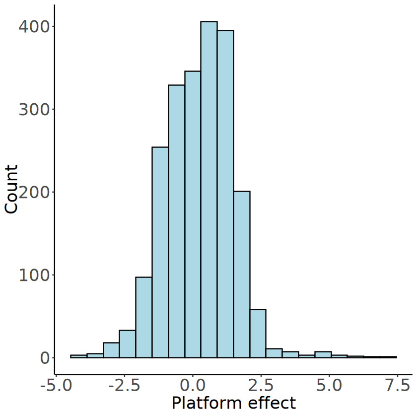
[9]:
# Platform effects
p <- ggplot(data = NULL, aes(x = platform_effects_ST[1, mcube_object@gene_test])) +
  geom_histogram(bins = 20, fill = "lightblue", color = "black") +
  xlab("Platform effect") +
  ylab("Count") +
  theme_classic() +
  theme(
    text = element_text(size = 20),
    axis.text = element_text(size = 20)
  )
ggsave(
  filename = file.path(RESULT_PATH, "platform_effects.pdf"),
  plot = p, width = 4, height = 4
)
p
[10]:
rm(mcube_object)
Visualization of the cell type-specific SVG results
[11]:
celltype <- "Ex_5_L5"
demo_genes <- c("COX6C", "CAMK2N1", "ENC1", "SYT1")
for(i in 1:n_slices){
    mcube_object <- get(paste0("mcube_object_", slice_idx_seq[i]))

    # Since STitch3D aligns multiple ST slices, the integrated 3D coordinates cannot match the H&E image
    # Therefore, we use the original 2D coordinates instead
    coordinates_original <- as.matrix(read.csv(
        file.path(DATA_PATH, paste0("2D_coordinates_slice", i - 1, ".csv")),
        header = TRUE, row.names = 1, check.names = FALSE
    ))
    rownames(coordinates_original) <- paste0(rownames(coordinates_original), "-slice", i - 1)
    coordinates_original <- coordinates_original[rownames(mcube_object@proportions), ]

    # Load in H&E image
    he_image <- tiff::readTIFF(
        file.path(
            RAW_DATA_PATH, "spatialLIBD", slice_idx_seq[i],
            paste0(slice_idx_seq[i], "_full_image.tif")
        )
    )
    he_image_0.5 <- array(0.5, dim = c(dim(he_image)[1], dim(he_image)[2], 4))
    he_image_0.5[, , 1] <- he_image[, , 1]
    he_image_0.5[, , 2] <- he_image[, , 2]
    he_image_0.5[, , 3] <- he_image[, , 3]
    # he_image_0.5[, , 4] <- 0.5

    boader <- 500
    xlim <- c(
        min(coordinates_original[, 1]) - boader,
        max(coordinates_original[, 1]) + boader
    )
    ylim <- c(
        min(coordinates_original[, 2]) - boader,
        max(coordinates_original[, 2]) + boader
    )

    # Proportions of cell type
    p1 <- mcubePlotPropCellType(
        mcube_object@proportions, coordinates_original, celltype,
        he_image = he_image_0.5[ylim[1]:ylim[2], xlim[1]:xlim[2], ],
        background = TRUE, opacity_background = 0,
        xlim = xlim, ylim = ylim
    ) +
      scale_x_continuous(limits = xlim, expand = c(0, 0)) +
        scale_y_continuous(trans = "reverse", limits = rev(ylim), expand = c(0, 0)) +
        scale_colour_gradientn(
            name = NULL,
            colors = pals::brewer.orrd(22)[3:22],
            breaks = c(0.10, 0.15, 0.20)
            ) +
        guides(color = guide_colorbar(barwidth = 15)) +
          theme_void() +
          theme(
            text = element_text(family = "Helvetica"),
              plot.title = element_blank(),
              axis.title = element_blank(),
              axis.text = element_blank(),
              axis.ticks = element_blank(),
              panel.grid = element_blank(),
              legend.position = "bottom",
              legend.title = element_blank(),
              legend.text = element_text(size = 20)
          )
    ggsave(
        filename = file.path(
            RESULT_PATH,
            paste0("proportion_", celltype, "_slice", slice_idx_seq[i], ".png")
        ),
        plot = p1, width = 4, height = 5, bg = "transparent"
    )
    ggsave(
        filename = file.path(
            RESULT_PATH,
            paste0("proportion_", celltype, "_slice", slice_idx_seq[i], ".pdf")
        ),
        plot = p1, width = 4, height = 5, bg = "transparent"
    )

    # Spatial pattern of SVGs
    for (gene in demo_genes) {
        mcube_object@coordinates <- coordinates_original
        p2 <- mcubePlotExprCellTypeBinary(
            mcube_object,
            celltype = celltype, gene = gene,
            he_image = he_image_0.5[ylim[1]:ylim[2], xlim[1]:xlim[2], ], background = FALSE,
            xlim = xlim, ylim = ylim
        ) +
        scale_x_continuous(limits = xlim, expand = c(0, 0)) +
        scale_y_continuous(trans = "reverse", limits = rev(ylim), expand = c(0, 0)) +
        guides(color = guide_legend(override.aes = list(size = 5))) +
                theme_void() +
                theme(
                    text = element_text(family = "Helvetica"),
                    plot.title = element_blank(),
                    axis.title = element_blank(),
                    axis.text = element_blank(),
                    axis.ticks = element_blank(),
                    panel.grid = element_blank(),
                    legend.position = "bottom",
                    legend.title = element_blank(),
                    legend.text = element_text(size = 20)
                )
        ggsave(
            filename = file.path(
                RESULT_PATH,
                paste0(celltype, "_", gene, "_slice", slice_idx_seq[i], ".png")
            ),
            plot = p2, width = 4, height = 5, bg = "transparent"
        )
        # ggsave(
        #     filename = file.path(
        #         RESULT_PATH,
        #         paste0(celltype, "_", gene, "_slice", slice_idx_seq[i], ".pdf")
        #     ),
        #     plot = p2, width = 4, height = 5, bg = "transparent"
        # )
    }

    rm(mcube_object)
}

p1
p2
Warning message in tiff::readTIFF(file.path(RAW_DATA_PATH, "spatialLIBD", slice_idx_seq[i], :
“TIFFReadDirectory: Unknown field with tag 40961 (0xa001) encountered”
Warning message in tiff::readTIFF(file.path(RAW_DATA_PATH, "spatialLIBD", slice_idx_seq[i], :
“TIFFReadDirectory: Unknown field with tag 65325 (0xff2d) encountered”
Warning message in tiff::readTIFF(file.path(RAW_DATA_PATH, "spatialLIBD", slice_idx_seq[i], :
“TIFFReadDirectory: Unknown field with tag 65326 (0xff2e) encountered”
Warning message in tiff::readTIFF(file.path(RAW_DATA_PATH, "spatialLIBD", slice_idx_seq[i], :
“TIFFReadDirectory: Unknown field with tag 65327 (0xff2f) encountered”
Warning message in tiff::readTIFF(file.path(RAW_DATA_PATH, "spatialLIBD", slice_idx_seq[i], :
“TIFFReadDirectory: Unknown field with tag 65329 (0xff31) encountered”
Warning message in tiff::readTIFF(file.path(RAW_DATA_PATH, "spatialLIBD", slice_idx_seq[i], :
“TIFFReadDirectory: Unknown field with tag 65330 (0xff32) encountered”
Warning message in tiff::readTIFF(file.path(RAW_DATA_PATH, "spatialLIBD", slice_idx_seq[i], :
“TIFFReadDirectory: Unknown field with tag 65331 (0xff33) encountered”
Warning message in tiff::readTIFF(file.path(RAW_DATA_PATH, "spatialLIBD", slice_idx_seq[i], :
“TIFFReadDirectory: Unknown field with tag 65332 (0xff34) encountered”
Warning message in tiff::readTIFF(file.path(RAW_DATA_PATH, "spatialLIBD", slice_idx_seq[i], :
“TIFFReadDirectory: Unknown field with tag 65333 (0xff35) encountered”
Scale for x is already present.
Adding another scale for x, which will replace the existing scale.
Scale for y is already present.
Adding another scale for y, which will replace the existing scale.
Scale for colour is already present.
Adding another scale for colour, which will replace the existing scale.
Scale for x is already present.
Adding another scale for x, which will replace the existing scale.
Scale for y is already present.
Adding another scale for y, which will replace the existing scale.
Scale for x is already present.
Adding another scale for x, which will replace the existing scale.
Scale for y is already present.
Adding another scale for y, which will replace the existing scale.
Scale for x is already present.
Adding another scale for x, which will replace the existing scale.
Scale for y is already present.
Adding another scale for y, which will replace the existing scale.
Scale for x is already present.
Adding another scale for x, which will replace the existing scale.
Scale for y is already present.
Adding another scale for y, which will replace the existing scale.
Warning message in tiff::readTIFF(file.path(RAW_DATA_PATH, "spatialLIBD", slice_idx_seq[i], :
“TIFFReadDirectory: Unknown field with tag 40961 (0xa001) encountered”
Warning message in tiff::readTIFF(file.path(RAW_DATA_PATH, "spatialLIBD", slice_idx_seq[i], :
“TIFFReadDirectory: Unknown field with tag 65325 (0xff2d) encountered”
Warning message in tiff::readTIFF(file.path(RAW_DATA_PATH, "spatialLIBD", slice_idx_seq[i], :
“TIFFReadDirectory: Unknown field with tag 65326 (0xff2e) encountered”
Warning message in tiff::readTIFF(file.path(RAW_DATA_PATH, "spatialLIBD", slice_idx_seq[i], :
“TIFFReadDirectory: Unknown field with tag 65327 (0xff2f) encountered”
Warning message in tiff::readTIFF(file.path(RAW_DATA_PATH, "spatialLIBD", slice_idx_seq[i], :
“TIFFReadDirectory: Unknown field with tag 65329 (0xff31) encountered”
Warning message in tiff::readTIFF(file.path(RAW_DATA_PATH, "spatialLIBD", slice_idx_seq[i], :
“TIFFReadDirectory: Unknown field with tag 65330 (0xff32) encountered”
Warning message in tiff::readTIFF(file.path(RAW_DATA_PATH, "spatialLIBD", slice_idx_seq[i], :
“TIFFReadDirectory: Unknown field with tag 65331 (0xff33) encountered”
Warning message in tiff::readTIFF(file.path(RAW_DATA_PATH, "spatialLIBD", slice_idx_seq[i], :
“TIFFReadDirectory: Unknown field with tag 65332 (0xff34) encountered”
Warning message in tiff::readTIFF(file.path(RAW_DATA_PATH, "spatialLIBD", slice_idx_seq[i], :
“TIFFReadDirectory: Unknown field with tag 65333 (0xff35) encountered”
Scale for x is already present.
Adding another scale for x, which will replace the existing scale.
Scale for y is already present.
Adding another scale for y, which will replace the existing scale.
Scale for colour is already present.
Adding another scale for colour, which will replace the existing scale.
Scale for x is already present.
Adding another scale for x, which will replace the existing scale.
Scale for y is already present.
Adding another scale for y, which will replace the existing scale.
Scale for x is already present.
Adding another scale for x, which will replace the existing scale.
Scale for y is already present.
Adding another scale for y, which will replace the existing scale.
Scale for x is already present.
Adding another scale for x, which will replace the existing scale.
Scale for y is already present.
Adding another scale for y, which will replace the existing scale.
Scale for x is already present.
Adding another scale for x, which will replace the existing scale.
Scale for y is already present.
Adding another scale for y, which will replace the existing scale.


Negative control using one slice
[12]:
mcube_object <- get(paste0("mcube_object_", slice_idx_seq[1]))

shuffle_idx <- sample(
    1:nrow(mcube_object@coordinates),
    nrow(mcube_object@coordinates)
)
write.csv(shuffle_idx, file = file.path(DATA_PATH, "shuffle_idx.csv"), row.names = FALSE)
shuffle_idx <- read.csv(file.path(DATA_PATH, "shuffle_idx.csv"), header = TRUE)[, 1]

coordinates_shuffle <- mcube_object@coordinates[shuffle_idx, ]
rownames(coordinates_shuffle) <- rownames(mcube_object@coordinates)
write.csv(coordinates_shuffle, file = file.path(DATA_PATH, "coordinates_shuffle.csv"))
coordinates_shuffle <- data.matrix(read.csv(
    file.path(DATA_PATH, "coordinates_shuffle.csv"),
    header = TRUE, row.names = 1, check.names = FALSE
))
[13]:
mcube_object_null <- mcube_object
rm(mcube_object)

mcube_object_null@coordinates <- coordinates_shuffle
mcube_object_null <- mcubeTest(
    mcube_object_null,
    num_workers = 70, num_threads = 1,
    shared_memory = TRUE
)

pvalues_null <- mcube_object_null@pvalues
rm(mcube_object_null)

p <- mcubePlotPvalues(
    pvalues_null, "combined_pvalue",
    nrow = 2, under_null = TRUE
) + labs(title = NULL) +
    theme(
        text = element_text(size = 16),
        plot.title = element_text(size = 20),
        axis.title = element_text(size = 20),
        axis.text.x = element_text(size = 16),
        axis.text.y = element_text(size = 16)
    )
ggsave(
    filename = file.path(
        RESULT_PATH,
        paste0("pvalue_qqplot_null_", slice_idx_seq[1], ".png")
    ),
    plot = p, width = 12, height = 7
)
p

saveRDS(
    pvalues_null,
    file = file.path(
        RESULT_PATH,
        paste0("pvalues_", slice_idx_seq[1], "_null.rds")
    )
)
# pvalues_null <- readRDS(
#     file = file.path(
#         RESULT_PATH,
#         paste0("pvalues_", slice_idx_seq[1], "_null.rds")
#     )
# )
mcubeKernel: length_scale is set as 0.10891969400686 for the Gaussian kernel.

mcubeKernel: length_scale is set as 0.154035708474029 for the Gaussian kernel.

mcubeKernel: length_scale is set as 0.10891969400686 for the Gaussian_transformed kernel.

mcubeKernel: length_scale is set as 0.154035708474029 for the Gaussian_transformed kernel.

Number of physical cores: 72.

Number of workers: 70.

Number of thread(s) on BLAS per worker: 1.

[14]:
rm(list = ls(pattern = "mcube_object_"))
Applying MCube to the integrated four ST slices together
[15]:
mcube_object_all <- createMCube(
    counts = counts, coordinates = coordinates,
    proportions = proportions_ST, library_sizes = library_sizes_ST,
    covariates = NULL, batch_id = batch_id,
    reference = reference_ST,
    spot_effects = spot_effects_ST, platform_effects = platform_effects_ST,
    project = "DLPFC_all"
)
mcube_object_all <- mcubeFitNull(
    mcube_object_all,
    num_workers = 35, num_threads = 2
)
mcube_object_all <- mcubeTest(
    mcube_object_all,
    num_workers = 35, num_threads = 2, shared_memory = TRUE
)

p <- mcubePlotPvalues(mcube_object_all@pvalues, "combined_pvalue", nrow = 3) +
    labs(title = NULL) +
    theme(
        text = element_text(size = 16),
        plot.title = element_text(size = 20),
        axis.title = element_text(size = 20),
        axis.text.x = element_text(size = 16),
        axis.text.y = element_text(size = 16)
    )
ggsave(
    filename = file.path(
        RESULT_PATH,
        paste0("pvalue_qqplot_all.png")
    ),
    plot = p, width = 12, height = 12
)
p
Select high-abundance cell types to analyze with proportion_threshold = 0.1 and celltype_threshold = 100.

mcubeFilterCellTypes: Cell type(s) Astros_3, Endo, Ex_10_L2_4, Ex_2_L5, Ex_3_L4_5, Ex_5_L5, Ex_6_L4_6, Ex_7_L4_6, Ex_8_L5_6, Micro/Macro, Oligos_1, Oligos_3 pass the threshold.

Cell type(s) Astros_1, Astros_2, Ex_1_L5_6, Ex_4_L_6, Ex_9_L5_6, Oligos_2 has/have less than the minimum celltype_threshold = 100 with proportion_threshold = 0.1.
To include the above cell type(s), please reduce celltype_threshold or proportion_threshold.

Cell type(s) Astros_3, Endo, Ex_10_L2_4, Ex_2_L5, Ex_3_L4_5, Ex_5_L5, Ex_6_L4_6, Ex_7_L4_6, Ex_8_L5_6, Micro/Macro, Oligos_1, Oligos_3 will be analyzed.

Filter out lowly-expressed genes with gene_threshold = 5e-05.

mcubeFilterGenes: 2208 genes pass the threshold.

Select highly-expressed genes to analyze for each specific cell type with reference_threshold = 0.5.

mcubeFilterGenesCellType: Select 590 genes to analyze for Astros_3.

mcubeFilterGenesCellType: Select 660 genes to analyze for Endo.

mcubeFilterGenesCellType: Select 627 genes to analyze for Ex_10_L2_4.

mcubeFilterGenesCellType: Select 916 genes to analyze for Ex_2_L5.

mcubeFilterGenesCellType: Select 778 genes to analyze for Ex_3_L4_5.

mcubeFilterGenesCellType: Select 976 genes to analyze for Ex_5_L5.

mcubeFilterGenesCellType: Select 594 genes to analyze for Ex_6_L4_6.

mcubeFilterGenesCellType: Select 608 genes to analyze for Ex_7_L4_6.

mcubeFilterGenesCellType: Select 618 genes to analyze for Ex_8_L5_6.

mcubeFilterGenesCellType: Select 504 genes to analyze for Micro/Macro.

mcubeFilterGenesCellType: Select 671 genes to analyze for Oligos_1.

mcubeFilterGenesCellType: Select 644 genes to analyze for Oligos_3.

Preprocessed data description: 14243 spots and 18 cell types in total. 14243 spots, 2205 genes, and 12 cell type(s) to analyze.

Number of physical cores: 72.

Number of workers: 35.

Number of thread(s) on BLAS per worker: 2.

mcubeKernel: length_scale is set as 0.0447877963411535 for the Gaussian kernel.

mcubeKernel: length_scale is set as 0.0633395090144634 for the Gaussian kernel.

mcubeKernel: length_scale is set as 0.0447877963411535 for the Gaussian_transformed kernel.

mcubeKernel: length_scale is set as 0.0633395090144634 for the Gaussian_transformed kernel.

Number of physical cores: 72.

Number of workers: 35.

Number of thread(s) on BLAS per worker: 2.

[16]:
saveRDS(
    mcube_object_all,
    file = file.path(
        RESULT_PATH,
        paste0("mcube_all", ".rds")
    )
)
# mcube_object_all <- readRDS(
#     file = file.path(
#         RESULT_PATH,
#         paste0("mcube_all", ".rds")
#     )
# )
Visualization of the cell type-specific SVG results from the 3D perspective
[17]:
# For visualization
mcube_object_all@coordinates[, "x"] = -mcube_object_all@coordinates[, "x"]
mcube_object_all@coordinates[, "z"] = (mcube_object_all@coordinates[, "z"] -
    (mcube_object_all@coordinates[, "z"] > 14) * 397.3) * 200
mcube_object_all@coordinates[, "x"] = mcube_object_all@coordinates[, "x"] / 1.37
mcube_object_all@coordinates[, "y"] = mcube_object_all@coordinates[, "y"] / 1.37
mcube_object_all@coordinates[, "z"] = mcube_object_all@coordinates[, "z"] / 1.37
[18]:
celltype <- "Ex_5_L5"
demo_genes <- c("COX6C", "CAMK2N1", "ENC1", "SYT1")
for (gene in demo_genes) {
    p <- mcubePlotExprCellType3D(
        mcube_object_all, celltype, gene,
        spot_size = 1.5, opacity_target = 0.7, opacity_background = 0.1,
        plotly_eye = list(x = -0.9, y = 1.7, z = 1.2)
    )
    plotly::save_image(
        p, file.path(RESULT_PATH, paste0(celltype, "_", gene, "_3D", ".pdf")),
        width = 500, height = 500, scale = 5
    )
}
Visualization of the platform effects across slices
[19]:
demo_genes <- c("COX6C", "CAMK2N1", "SYT1")
n_slices <- 4
n_genes <- 3
platform_effects_demo_gene <- data.frame(
    slice = rep(paste("Slice", slice_idx_seq), n_genes),
    gene = rep(demo_genes, each = n_slices),
    platform_effect = as.vector(platform_effects_ST[, demo_genes])
)
platform_effects_demo_gene$gene <- factor(
    platform_effects_demo_gene$gene,
    levels = demo_genes
)
[20]:
p <- ggplot(data = platform_effects_demo_gene, aes(x = slice, y = platform_effect)) +
    geom_bar(stat = "identity", fill = "dodgerblue") +
    labs(x = NULL, y = "Platform effect") +
    facet_wrap(vars(gene), nrow = 1, scales = "free_y") +
    theme_classic() +
    theme(
        axis.title = element_text(size = 20),
        axis.text.x = element_text(size = 12, angle = 45, hjust = 1),
        axis.text.y = element_text(size = 16),
        strip.text = element_text(size = 12, face = "italic")
    )
ggsave(
    filename = file.path(
        RESULT_PATH,
        paste0(
            "batch_effects",
            ".pdf"
        )
    ),
    plot = p, width = 10, height = 4
)
p

Comparison of the 2D and 3D results
[21]:
celltype <- "Ex_5_L5"
for (i in 1:n_slices) {
    mcube_object <- readRDS(
        file = file.path(
            RESULT_PATH,
            paste0("mcube_", slice_idx_seq[i], ".rds")
        )
    )
    assign(
        paste0("svg_list_", i),
        mcubeGetSigGenes(mcube_object@pvalues)[[celltype]]
    )
}
svg_list_all <- mcubeGetSigGenes(mcube_object_all@pvalues)[[celltype]]
mcubeGetSigGenes: Set adjust_method as BH and alpha as 0.05.

mcubeGetSigGenes: Set adjust_method as BH and alpha as 0.05.

mcubeGetSigGenes: Set adjust_method as BH and alpha as 0.05.

mcubeGetSigGenes: Set adjust_method as BH and alpha as 0.05.

mcubeGetSigGenes: Set adjust_method as BH and alpha as 0.05.
[22]:
svg_list <- list(
    All_slices = rownames(svg_list_all),
    Slice_1 = rownames(svg_list_1),
    Slice_2 = rownames(svg_list_2),
    Slice_3 = rownames(svg_list_3),
    Slice_4 = rownames(svg_list_4)
)
names(svg_list) <- c("All slices", paste("Slice", slice_idx_seq))
[23]:
all_genes <- unique(unlist(svg_list))
svg_mat <- matrix(FALSE, nrow = length(all_genes), ncol = length(svg_list))
rownames(svg_mat) <- all_genes
colnames(svg_mat) <- names(svg_list)

for (i in 1:length(svg_list)) {
    svg_mat[svg_list[[i]], i] <- TRUE
}
head(svg_mat)
| All slices | Slice 151673 | Slice 151674 | Slice 151675 | Slice 151676 | |
|---|---|---|---|---|---|
| COX6C | TRUE | TRUE | TRUE | TRUE | TRUE |
| CAMK2N1 | TRUE | TRUE | TRUE | TRUE | TRUE |
| TUBA1B | TRUE | TRUE | TRUE | TRUE | TRUE |
| ENC1 | TRUE | TRUE | TRUE | TRUE | TRUE |
| SYT1 | TRUE | TRUE | TRUE | TRUE | TRUE |
| TMSB10 | TRUE | TRUE | TRUE | TRUE | TRUE |
[24]:
# "#e07a5f","#3d405b","#81b29a","#f2cc8f"
library(ComplexUpset)
p <- upset(
    data = as.data.frame(svg_mat),
    intersect = rev(colnames(svg_mat)),
    max_degree = 2,
    sort_sets = FALSE,
    group_by = "sets",
    mode = 'inclusive_intersection',
    queries = list(
        upset_query(group = names(svg_list)[1], color = "black"),
        upset_query(group = names(svg_list)[2], color = "#e07a5f"),
        upset_query(group = names(svg_list)[3], color = "#3d405b"),
        upset_query(group = names(svg_list)[4], color = "#81b29a"),
        upset_query(group = names(svg_list)[5], color = "#f2cc8f"),
        upset_query(set = names(svg_list)[1], fill = "black"),
        upset_query(set = names(svg_list)[2], fill = "#e07a5f"),
        upset_query(set = names(svg_list)[3], fill = "#3d405b"),
        upset_query(set = names(svg_list)[4], fill = "#81b29a"),
        upset_query(set = names(svg_list)[5], fill = "#f2cc8f")
    )
) + theme_classic()
ggsave(
    file.path(RESULT_PATH, "upset.pdf"),
    plot = p, width = 10, height = 6
)
p
