Comparison with the methods not considering cell type mixtures
[1]:
set.seed(20240709)

library(MCube)
library(SPARK)
library(HEARTSVG)
library(ggplot2)

max_cores <- 8
[2]:
RAW_DATA_PATH <- "/import/home/share/zw/data/DLPFC"
DATA_PATH <- "/import/home/share/zw/pql/data/DLPFC"
RESULT_PATH <- "/import/home/share/zw/pql/results/DLPFC"

if (!dir.exists(file.path(RESULT_PATH))) {
    dir.create(file.path(RESULT_PATH), recursive = TRUE)
}
[3]:
# Use Slice 151673 as an example
slice_idx <- 151673

# Load in ST data
counts <- as.data.frame(readr::read_csv(file.path(DATA_PATH, "counts.csv")))
rownames(counts) <- counts[, 1]
counts[, 1] <- NULL
counts <- as.matrix(counts)
spots_names <- grep("-slice0$", rownames(counts), value = TRUE) # Spots at the first slice
counts <- counts[spots_names, ]
dim(counts)
# head(counts)
coordinates <- as.data.frame(readr::read_csv(file.path(DATA_PATH, "3D_coordinates.csv")))
rownames(coordinates) <- coordinates[, 1]
coordinates[, c(1, 4)] <- NULL
coordinates <- coordinates[spots_names, ]
dim(coordinates)
# head(coordinates)
New names:
• `` -> `...1`
Rows: 14243 Columns: 4559
── Column specification ────────────────────────────────────────────────────────
Delimiter: ","
chr    (1): ...1
dbl (4558): A2M, AAK1, AASDHPPT, AASS, AATK, ABCA1, ABCA2, ABCA5, ABCA8, ABC...

ℹ Use `spec()` to retrieve the full column specification for this data.
ℹ Specify the column types or set `show_col_types = FALSE` to quiet this message.
- 3611
- 4558
New names:
• `` -> `...1`
Rows: 14243 Columns: 4
── Column specification ────────────────────────────────────────────────────────
Delimiter: ","
chr (1): ...1
dbl (3): x, y, z

ℹ Use `spec()` to retrieve the full column specification for this data.
ℹ Specify the column types or set `show_col_types = FALSE` to quiet this message.
- 3611
- 2
Methods not considering cell type mixtures
SPARK and SPARK-X (https://github.com/xzhoulab/SPARK)
[4]:
spark_obj <- CreateSPARKObject(counts = t(counts), location = coordinates)
spark_obj@lib_size <- rowSums(counts)

spark_obj <- spark.vc(
    spark_obj,
    covariates = NULL, lib_size = spark_obj@lib_size,
    num_core = max_cores, verbose = FALSE
)
spark_obj <- spark.test(spark_obj, check_positive = TRUE, verbose = FALSE)

saveRDS(spark_obj, file = file.path(RESULT_PATH, "spark.rds"))
## ===== SPARK INPUT INFORMATION ====
## number of total samples:  3611
## number of total features:  2049
## number of adjusted covariates:  0
# fitting count-based spatial model under the null hypothesis ...
## testing Gaussian kernel: 1...
## testing Periodic kernel: 1...
## testing Gaussian kernel: 2...
## testing Periodic kernel: 2...
## testing Gaussian kernel: 3...
## testing Periodic kernel: 3...
## testing Gaussian kernel: 4...
## testing Periodic kernel: 4...
## testing Gaussian kernel: 5...
## testing Periodic kernel: 5...
[5]:
sparkx_results <- sparkx(t(counts), as.matrix(coordinates), numCores = max_cores, option = "mixture")
saveRDS(sparkx_results, file = file.path(RESULT_PATH, "sparkx.rds"))
## ===== SPARK-X INPUT INFORMATION ====
## number of total samples: 3611
## number of total genes: 4216
## Running with 8 cores
## Testing With Projection Kernel
## Testing With Gaussian Kernel 1
## Testing With Gaussian Kernel 2
## Testing With Gaussian Kernel 3
## Testing With Gaussian Kernel 4
## Testing With Gaussian Kernel 5
## Testing With Cosine Kernel 1
## Testing With Cosine Kernel 2
## Testing With Cosine Kernel 3
## Testing With Cosine Kernel 4
## Testing With Cosine Kernel 5
HEARTSVG (https://github.com/cz0316/HEARTSVG)
[6]:
heartsvg_data <- cbind(coordinates, counts)
colnames(heartsvg_data)[1:2] <- c("row", "col")

heartsvg_results <- heartsvg(heartsvg_data, scale = TRUE)

write.csv(heartsvg_results,file.path(RESULT_PATH, "heartsvg_results.csv"))
Comparison of the SVG identification results
[7]:
# Load in SVG identification results
spark_obj <- readRDS(file.path(RESULT_PATH, "spark.rds"))
sparkx_results <- readRDS(file.path(RESULT_PATH, "sparkx.rds"))
heartsvg_results <- read.csv(file.path(RESULT_PATH, "heartsvg_results.csv"), row.names = 1)
rownames(heartsvg_results) <- heartsvg_results$gene
[8]:
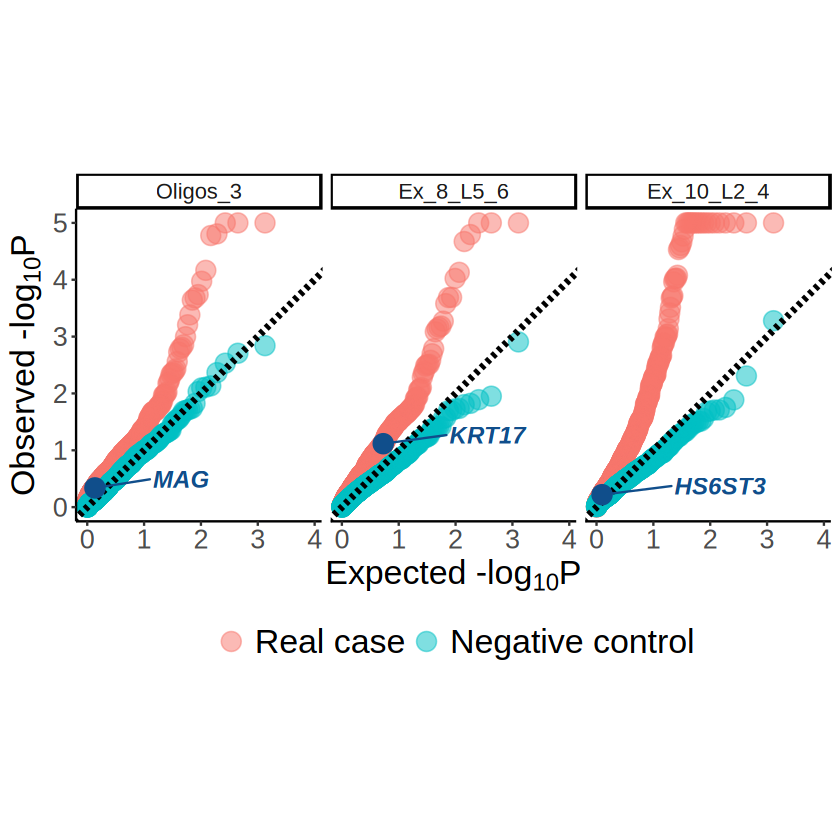
demo_celltypes <- c("Oligos_3", "Ex_8_L5_6", "Ex_10_L2_4")
markers <- c("MAG", "KRT17", "HS6ST3")
[9]:
others_pvalues_long <- rbind(
    data.frame(
        method = "SPARK",
        mcubeQQPlotDF(spark_obj@res_mtest, "combined_pvalue")
    ),
    data.frame(
        method = "SPARK-X",
        mcubeQQPlotDF(sparkx_results$res_mtest, "combinedPval")
    ),
    data.frame(
        method = "HEARTSVG",
        mcubeQQPlotDF(heartsvg_results, "p_adj")
    )
)
others_pvalues_long$case <- "Real case"
others_pvalues_long$case <- factor(others_pvalues_long$case, levels = c("Real case", "Negative control"))
# dim(others_pvalues_long)
# head(others_pvalues_long)

others_marker_pvalues <- others_pvalues_long[others_pvalues_long$gene %in% markers, ]
others_marker_pvalues
| method | gene | pvalue | pvalue_theoretical | minus_log10p | minus_log10p_theoretical | case | |
|---|---|---|---|---|---|---|---|
| <chr> | <chr> | <dbl> | <dbl> | <dbl> | <dbl> | <fct> | |
| 350 | SPARK | HS6ST3 | 5.550000e-17 | 0.17057101 | 5 | 0.7680948 | Real case |
| 400 | SPARK | KRT17 | 5.550000e-17 | 0.19497316 | 5 | 0.7100252 | Real case |
| 996 | SPARK | MAG | 2.220446e-16 | 0.48584675 | 5 | 0.3135007 | Real case |
| 2105 | SPARK-X | MAG | 3.821175e-189 | 0.01316414 | 5 | 1.8806076 | Real case |
| 2642 | SPARK-X | HS6ST3 | 5.262656e-74 | 0.14053605 | 5 | 0.8522122 | Real case |
| 3218 | SPARK-X | KRT17 | 9.791988e-33 | 0.27715844 | 5 | 0.5572719 | Real case |
| 7017 | HEARTSVG | MAG | 0.000000e+00 | 0.17824953 | 5 | 0.7489716 | Real case |
| 7148 | HEARTSVG | HS6ST3 | 0.000000e+00 | 0.20932163 | 5 | 0.6791859 | Real case |
| 7169 | HEARTSVG | KRT17 | 0.000000e+00 | 0.21430266 | 5 | 0.6689724 | Real case |
The cell type marker genes are identified as SVGs by the methods not considering cell type mixtures.
[10]:
expected_minus_log10p_lab <- expression(paste("Expected -log"[10], plain(P)))
observed_minus_log10p_lab <- expression(paste("Observed -log"[10], plain(P)))

x_max <- max(others_pvalues_long$minus_log10p_theoretical)

p <- ggplot(
    data = others_pvalues_long,
    aes(x = minus_log10p_theoretical, y = minus_log10p)
) +
    geom_point(aes(color = case), alpha = 0.5, size = 5) +
    geom_abline(
        intercept = 0, slope = 1, linewidth = 1.5,
        linetype = "dashed", color = "black"
    ) +
    geom_point(data = others_marker_pvalues, color = "dodgerblue4", size = 5, alpha = 1) +
    ggrepel::geom_text_repel(
        data = others_marker_pvalues, aes(label = gene),
        color = "dodgerblue4", size = 5, fontface = "bold.italic",
        angle=0, direction = 'y', vjust=0, point.size = 5
    ) +
    xlim(0, x_max) +
    coord_fixed(ratio = 1) +
    facet_wrap(~ factor(method, c("SPARK", "SPARK-X", "HEARTSVG")), nrow = 1) +
    labs(
        title = NULL,
        x = expected_minus_log10p_lab, y = observed_minus_log10p_lab
    ) +
    theme_classic() +
    theme(
        text = element_text(family = "Helvetica", size = 16),
        plot.title = element_text(size = 20),
        axis.title = element_text(size = 20),
        axis.text.x = element_text(size = 16),
        axis.text.y = element_text(size = 16),
        legend.position = "none"
    )
ggsave(
    filename = file.path(RESULT_PATH, "others_marker.pdf"),
    plot = p, width = 8, height = 4
)
p

[11]:
# Load in MCube results
mcube_object <- readRDS(file.path(RESULT_PATH, paste0("mcube_", slice_idx, ".rds")))
mcube_pvalues <- mcube_object@pvalues
mcube_pvalues_null <- readRDS(file.path(RESULT_PATH, paste0("pvalues_", slice_idx, "_null.rds")))
[12]:
mcube_pvalues_long <- rbind(
    do.call(
        rbind,
        lapply(
            names(mcube_pvalues),
            FUN = function(x) {
                data.frame(
                    celltype = x,
                    mcubeQQPlotDF(mcube_pvalues[[x]]),
                    case = "Real case"
                )
            }
        )
    ),
    do.call(
        rbind,
        lapply(
            names(mcube_pvalues_null),
            FUN = function(x) {
                data.frame(
                    celltype = x,
                    mcubeQQPlotDF(mcube_pvalues_null[[x]]),
                    case = "Negative control"
                )
            }
        )
    )
)
mcube_pvalues_long$case <- factor(mcube_pvalues_long$case, levels = c("Real case", "Negative control"))
mcube_pvalues_long <- mcube_pvalues_long[mcube_pvalues_long$celltype %in% demo_celltypes, ]
# head(mcube_pvalues_long)

mcube_marker_pvalues <- mcube_pvalues_long[
    mcube_pvalues_long$gene %in% markers & mcube_pvalues_long$case == "Real case",
]
mcube_marker_pvalues
| celltype | gene | pvalue | pvalue_theoretical | minus_log10p | minus_log10p_theoretical | case | |
|---|---|---|---|---|---|---|---|
| <chr> | <chr> | <dbl> | <dbl> | <dbl> | <dbl> | <fct> | |
| 1157 | Ex_10_L2_4 | HS6ST3 | 0.6041588 | 0.7992308 | 0.2188489 | 0.0973278 | Real case |
| 4036 | Ex_8_L5_6 | KRT17 | 0.0765885 | 0.1873041 | 1.1158364 | 0.7274528 | Real case |
| 5748 | Oligos_3 | MAG | 0.4591788 | 0.7320896 | 0.3380182 | 0.1354358 | Real case |
[13]:
# x_max <- max(mcube_pvalues_long$minus_log10p_theoretical)

p <- ggplot(
    data = mcube_pvalues_long, aes(x = minus_log10p_theoretical, y = minus_log10p)
) +
    geom_point(alpha = 0.5, aes(color = case), size = 5) +
    scale_color_discrete(name = "Case", labels = c("Real case", "Negative control")) +
    geom_abline(
        intercept = 0, slope = 1, linewidth = 1.5,
        linetype = "dashed", color = "black"
    ) +
    geom_point(data = mcube_marker_pvalues, color = "dodgerblue4", size = 5, alpha = 1) +
    ggrepel::geom_text_repel(
        data = mcube_marker_pvalues, aes(label = gene),
        color = "dodgerblue4", size = 5, fontface = "bold.italic",
        angle = 0, hjust = -0.5, vjust = 0, nudge_x = 0.5, point.size = 5
    ) +
    xlim(0, x_max) +
    coord_fixed(ratio = 1) +
    facet_wrap(~ factor(celltype, c("Oligos_3", "Ex_8_L5_6", "Ex_10_L2_4")), nrow = 1) +
    labs(
        title = NULL,
        x = expected_minus_log10p_lab, y = observed_minus_log10p_lab
    ) +
    theme_classic() +
    theme(
        text = element_text(family = "Helvetica", size = 16),
        plot.title = element_text(size = 20),
        axis.title = element_text(size = 20),
        axis.text.x = element_text(size = 16),
        axis.text.y = element_text(size = 16),
        legend.position = "bottom",
        legend.title = element_blank(),
        legend.text = element_text(size = 20)
    )
ggsave(
    file.path(RESULT_PATH, "MCube_marker.pdf"),
    plot = p, width = 8, height = 4
)
p
[14]:
# Load in H&E image
he_image <- tiff::readTIFF(
    file.path(
        RAW_DATA_PATH, "spatialLIBD", slice_idx,
        paste0(slice_idx, "_full_image.tif")
    )
)
he_image_0.5 <- array(0.5, dim = c(dim(he_image)[1], dim(he_image)[2], 4))
he_image_0.5[, , 1] <- he_image[, , 1]
he_image_0.5[, , 2] <- he_image[, , 2]
he_image_0.5[, , 3] <- he_image[, , 3]
# he_image_0.5[, , 4] <- 0.5

boader <- 500
xlim <- c(
    min(mcube_object@coordinates[, 1]) - boader,
    max(mcube_object@coordinates[, 1]) + boader
)
ylim <- c(
    min(mcube_object@coordinates[, 2]) - boader,
    max(mcube_object@coordinates[, 2]) + boader
)
Warning message in tiff::readTIFF(file.path(RAW_DATA_PATH, "spatialLIBD", slice_idx, :
“TIFFReadDirectory: Unknown field with tag 40961 (0xa001) encountered”
Warning message in tiff::readTIFF(file.path(RAW_DATA_PATH, "spatialLIBD", slice_idx, :
“TIFFReadDirectory: Unknown field with tag 65325 (0xff2d) encountered”
Warning message in tiff::readTIFF(file.path(RAW_DATA_PATH, "spatialLIBD", slice_idx, :
“TIFFReadDirectory: Unknown field with tag 65326 (0xff2e) encountered”
Warning message in tiff::readTIFF(file.path(RAW_DATA_PATH, "spatialLIBD", slice_idx, :
“TIFFReadDirectory: Unknown field with tag 65327 (0xff2f) encountered”
Warning message in tiff::readTIFF(file.path(RAW_DATA_PATH, "spatialLIBD", slice_idx, :
“TIFFReadDirectory: Unknown field with tag 65329 (0xff31) encountered”
Warning message in tiff::readTIFF(file.path(RAW_DATA_PATH, "spatialLIBD", slice_idx, :
“TIFFReadDirectory: Unknown field with tag 65330 (0xff32) encountered”
Warning message in tiff::readTIFF(file.path(RAW_DATA_PATH, "spatialLIBD", slice_idx, :
“TIFFReadDirectory: Unknown field with tag 65331 (0xff33) encountered”
Warning message in tiff::readTIFF(file.path(RAW_DATA_PATH, "spatialLIBD", slice_idx, :
“TIFFReadDirectory: Unknown field with tag 65332 (0xff34) encountered”
Warning message in tiff::readTIFF(file.path(RAW_DATA_PATH, "spatialLIBD", slice_idx, :
“TIFFReadDirectory: Unknown field with tag 65333 (0xff35) encountered”
[15]:
for (i in 1:3) {
    celltype <- demo_celltypes[i]
    gene <- markers[i]

    # Proportion of cell type
    p1 <- mcubePlotPropCellType(
        mcube_object@proportions, mcube_object@coordinates, celltype,
        he_image = he_image_0.5[ylim[1]:ylim[2], xlim[1]:xlim[2], ],
        background = TRUE, opacity_background = 0,
        xlim = xlim, ylim = ylim
    ) + scale_x_continuous(limits = xlim, expand = c(0, 0)) +
        scale_y_continuous(trans = "reverse", limits = rev(ylim), expand = c(0, 0)) +
        scale_colour_gradientn(
            name = NULL,
            colors = pals::brewer.orrd(22)[3:22],
            breaks = c(0.2, 0.4, 0.6)
            ) +
        guides(color = guide_colorbar(barwidth = 15)) +
        theme_void() +
        theme(
            text = element_text(family = "Helvetica"),
            plot.title = element_blank(),
            axis.title = element_blank(),
            axis.text = element_blank(),
            axis.ticks = element_blank(),
            panel.grid = element_blank(),
            legend.position = "bottom",
            legend.title = element_blank(),
            legend.text = element_text(size = 20)
        )
    ggsave(
        filename = file.path(
            RESULT_PATH,
            paste0("proportion_", celltype, "_slice", slice_idx, ".png")
        ),
        plot = p1, width = 4, height = 5, bg = "transparent"
    )

    # Gene expression
    p2 <- mcubePlotExpr(
        mcube_object@counts, mcube_object@coordinates, gene,
        he_image = he_image_0.5[ylim[1]:ylim[2], xlim[1]:xlim[2], ], background = FALSE,
        xlim = xlim, ylim = ylim, palettes = pals::brewer.bugn(20)[11:20]
    ) +
        scale_x_continuous(limits = xlim, expand = c(0, 0)) +
            scale_y_continuous(trans = "reverse", limits = rev(ylim), expand = c(0, 0)) +
            scale_colour_gradientn(
      name = NULL,
       colors = pals::brewer.bugn(20)[11:20],
breaks = c(0.4,0.6,0.8)
    ) +
            guides(color = guide_colorbar(barwidth = 15)) +
            theme_void() +
            theme(
                text = element_text(family = "Helvetica"),
                plot.title = element_blank(),
                axis.title = element_blank(),
                axis.text = element_blank(),
                axis.ticks = element_blank(),
                panel.grid = element_blank(),
                legend.position = "bottom",
                legend.title = element_blank(),
                legend.text = element_text(size = 20)
            )
    ggsave(
        filename = file.path(
            RESULT_PATH,
            paste0(gene, "_slice", slice_idx, ".png")
        ),
        plot = p2, width = 4, height = 5, bg = "transparent"
    )

    # Cell-type-specific gene expression variations
    p3 <- mcubePlotExprCellTypeBinary(
        mcube_object,
        celltype = celltype, gene = gene,
        he_image = he_image_0.5[ylim[1]:ylim[2], xlim[1]:xlim[2], ], background = FALSE,
        xlim = xlim, ylim = ylim
    ) +
    scale_x_continuous(limits = xlim, expand = c(0, 0)) +
    scale_y_continuous(trans = "reverse", limits = rev(ylim), expand = c(0, 0)) +
    guides(color = guide_legend(override.aes = list(size = 5))) +
    theme_void() +
    theme(
        text = element_text(family = "Helvetica"),
        plot.title = element_blank(),
        axis.title = element_blank(),
        axis.text = element_blank(),
        axis.ticks = element_blank(),
        panel.grid = element_blank(),
        legend.position = "bottom",
        legend.title = element_blank(),
        legend.text = element_text(size = 20)
    )
    ggsave(
        filename = file.path(
            RESULT_PATH,
            paste0(celltype, "_", gene, "_slice", slice_idx, ".png")
        ),
        plot = p3, width = 4, height = 5, bg = "transparent"
    )
}

p1
p2
p3
Scale for x is already present.
Adding another scale for x, which will replace the existing scale.
Scale for y is already present.
Adding another scale for y, which will replace the existing scale.
Scale for colour is already present.
Adding another scale for colour, which will replace the existing scale.
Scale for x is already present.
Adding another scale for x, which will replace the existing scale.
Scale for y is already present.
Adding another scale for y, which will replace the existing scale.
Scale for x is already present.
Adding another scale for x, which will replace the existing scale.
Scale for y is already present.
Adding another scale for y, which will replace the existing scale.
Scale for colour is already present.
Adding another scale for colour, which will replace the existing scale.
Scale for x is already present.
Adding another scale for x, which will replace the existing scale.
Scale for y is already present.
Adding another scale for y, which will replace the existing scale.
Scale for x is already present.
Adding another scale for x, which will replace the existing scale.
Scale for y is already present.
Adding another scale for y, which will replace the existing scale.
Scale for colour is already present.
Adding another scale for colour, which will replace the existing scale.
Scale for x is already present.
Adding another scale for x, which will replace the existing scale.
Scale for y is already present.
Adding another scale for y, which will replace the existing scale.
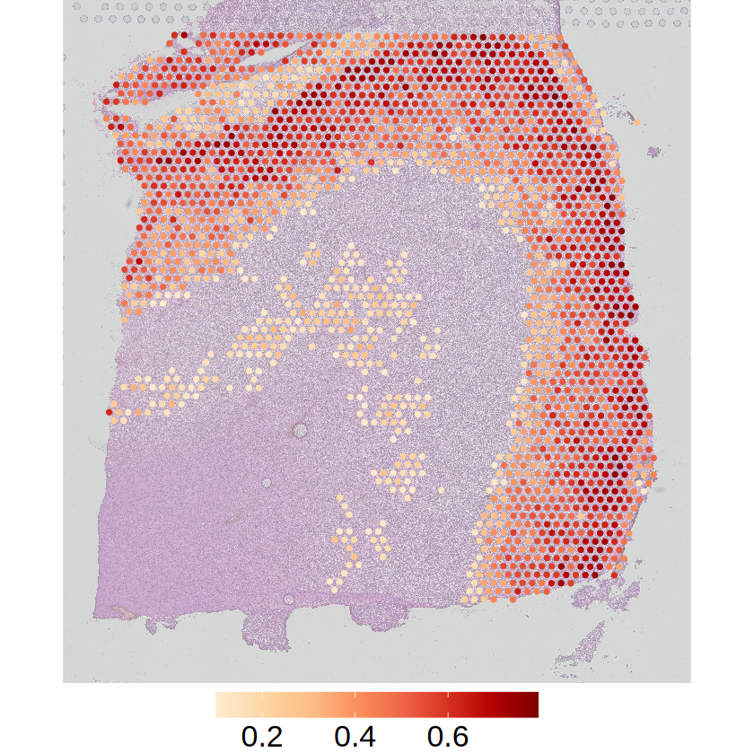
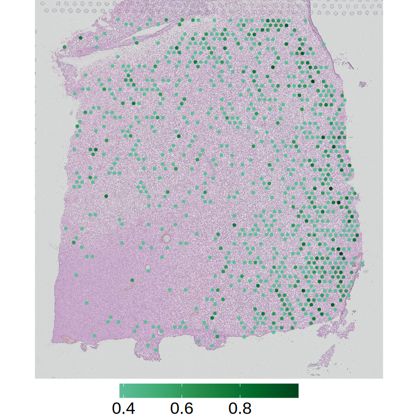
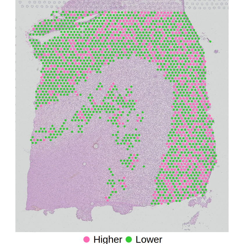
The spatial expression patterns of these marker genes are mainly affected by the distribution of cell type proportions across space. MCube results reveal that their spatial variations are evenly distributed within a specific cell type by accounting for the cell type composition, and thus not cell-type-specific SVGs.