Applying MCube to multiple adult mouse brain datasets from different sources
[1]:
set.seed(20240709)
library(MCube)
library(ggplot2)
library(tidyverse)
── Attaching core tidyverse packages ──────────────────────── tidyverse 2.0.0 ──
✔ dplyr 1.1.4 ✔ readr 2.1.5
✔ forcats 1.0.0 ✔ stringr 1.5.1
✔ lubridate 1.9.4 ✔ tibble 3.2.1
✔ purrr 1.0.4 ✔ tidyr 1.3.1
── Conflicts ────────────────────────────────────────── tidyverse_conflicts() ──
✖ dplyr::filter() masks stats::filter()
✖ dplyr::lag() masks stats::lag()
ℹ Use the conflicted package (<http://conflicted.r-lib.org/>) to force all conflicts to become errors
[2]:
DATA_PATH <- "/import/home/share/zw/pql/data/mouse_brain"
RESULT_PATH <- "/import/home/share/zw/pql/results/mouse_brain"
if (!dir.exists(file.path(RESULT_PATH, "visium_1"))) {
dir.create(file.path(RESULT_PATH, "visium_1"), recursive = TRUE)
}
if (!dir.exists(file.path(RESULT_PATH, "visium_2"))) {
dir.create(file.path(RESULT_PATH, "visium_2"), recursive = TRUE)
}
if (!dir.exists(file.path(RESULT_PATH, "ST_3D"))) {
dir.create(file.path(RESULT_PATH, "ST_3D"), recursive = TRUE)
}
Two slices of the Visium dataset
Visium Slice 1
[3]:
reference_ST <- data.matrix(read.csv(
file.path(DATA_PATH, "visium_1", "reference_ST.csv"),
header = TRUE, row.names = 1, check.names = FALSE
))
dim(reference_ST)
num_celltypes <- nrow(reference_ST)
proportions_ST <- data.matrix(read.csv(
file.path(DATA_PATH, "visium_1", paste0("prop_slice", 0, ".csv")),
header = TRUE, row.names = 1, check.names = FALSE
))
dim(proportions_ST)
counts <- as.data.frame(readr::read_csv(
file.path(DATA_PATH, "visium_1", "counts.csv")
))
rownames(counts) <- counts[, 1]
counts[, 1] <- NULL
counts <- data.matrix(counts)
dim(counts)
coordinates <- data.matrix(read.csv(
file.path(DATA_PATH, "visium_1", "3D_coordinates.csv"),
header = TRUE, row.names = 1, check.names = FALSE
))[, c("x", "y")]
shuffle_idx <- sample(1:nrow(coordinates), nrow(coordinates))
write.csv(shuffle_idx, file = file.path(DATA_PATH, "visium_1", "shuffle_idx.csv"), row.names = FALSE)
shuffle_idx <- read.csv(file.path(DATA_PATH, "visium_1", "shuffle_idx.csv"), header = TRUE)[, 1]
length(unique(shuffle_idx))
coordinates_shuffle <- coordinates[shuffle_idx, ]
rownames(coordinates_shuffle) <- rownames(coordinates)
write.csv(coordinates_shuffle, file = file.path(DATA_PATH, "visium_1", "coordinates_shuffle.csv"))
coordinates_shuffle <- data.matrix(read.csv(
file.path(DATA_PATH, "visium_1", "coordinates_shuffle.csv"),
header = TRUE, row.names = 1, check.names = FALSE
))
dim(coordinates)
dim(coordinates_shuffle)
spot_effects_ST <- data.matrix(read.csv(
file.path(DATA_PATH, "visium_1", "spot_effects_ST.csv"),
header = TRUE, row.names = 1, check.names = FALSE
))[, 1]
library_sizes_ST <- data.matrix(read.csv(
file.path(DATA_PATH, "visium_1", "library_sizes_ST.csv"),
header = TRUE, row.names = 1, check.names = FALSE
))[, 1]
- 59
- 6415
- 4168
- 59
New names:
• `` -> `...1`
Rows: 4168 Columns: 6416
── Column specification ────────────────────────────────────────────────────────
Delimiter: ","
chr (1): ...1
dbl (6415): 0610040J01Rik, 0610043K17Rik, 1110002J07Rik, 1110004F10Rik, 1110...
ℹ Use `spec()` to retrieve the full column specification for this data.
ℹ Specify the column types or set `show_col_types = FALSE` to quiet this message.
- 4168
- 6415
4168
- 4168
- 2
- 4168
- 2
[4]:
# Real case
mcube_object_1 <- createMCube(
counts = counts, coordinates = coordinates,
proportions = proportions_ST, library_sizes = library_sizes_ST,
covariates = NULL,
reference = reference_ST,
spot_effects = spot_effects_ST, platform_effects = NULL,
project = "mouse_brain_visium_1"
)
mcube_object_1 <- mcubeFitNull(
mcube_object_1,
num_workers = 70, num_threads = 1
)
mcube_object_1 <- mcubeTest(
mcube_object_1,
num_workers = 70, num_threads = 1, shared_memory = TRUE
)
p <- mcubePlotPvalues(mcube_object_1@pvalues, "combined_pvalue", nrow = 2)
p <- p +
labs(title = "10x Visium Slice 1") +
theme(
text = element_text(size = 16),
plot.title = element_text(size = 20),
axis.title = element_text(size = 20),
axis.text.x = element_text(size = 16),
axis.text.y = element_text(size = 16)
)
p
ggsave(
filename = file.path(
RESULT_PATH, "visium_1",
paste0("pvalue_qqplot.png")
),
plot = p, width = 12, height = 7
)
The batch_id is not provided!
All spots are assumed to be from the same batch and share the same gene platform effects.
Select high-abundance cell types to analyze with proportion_threshold = 0.1 and celltype_threshold = 100.
mcubeFilterCellTypes: Cell type(s) Ext_Hpc_CA1, Ext_Hpc_DG1, Ext_L23, Ext_L5_1, Ext_Pir, Ext_Thal_1, Ext_Thal_2, Inh_1, Inh_4, Oligo_2 pass the threshold.
Cell type(s) Astro_AMY, Astro_AMY_CTX, Astro_CTX, Astro_HPC, Astro_HYPO, Astro_STR, Astro_THAL_hab, Astro_THAL_lat, Astro_THAL_med, Astro_WM, Endo, Ext_Amy_1, Ext_Amy_2, Ext_ClauPyr, Ext_Hpc_CA2, Ext_Hpc_CA3, Ext_Hpc_DG2, Ext_L25, Ext_L56, Ext_L5_2, Ext_L5_3, Ext_L6, Ext_L6B, Ext_Med, Ext_Unk_1, Ext_Unk_2, Ext_Unk_3, Inh_2, Inh_3, Inh_5, Inh_6, Inh_Lamp5, Inh_Meis2_1, Inh_Meis2_2, Inh_Meis2_3, Inh_Meis2_4, Inh_Pvalb, Inh_Sst, Inh_Vip, LowQ_1, LowQ_2, Micro, Nb_1, Nb_2, OPC_1, OPC_2, Oligo_1, Unk_1, Unk_2 has/have less than the minimum celltype_threshold = 100 with proportion_threshold = 0.1.
To include the above cell type(s), please reduce celltype_threshold or proportion_threshold.
Cell type(s) Ext_Hpc_CA1, Ext_Hpc_DG1, Ext_L23, Ext_L5_1, Ext_Pir, Ext_Thal_1, Ext_Thal_2, Inh_1, Inh_4, Oligo_2 will be analyzed.
Filter out lowly-expressed genes with gene_threshold = 5e-05.
mcubeFilterGenes: 2768 genes pass the threshold.
The platform effects are not provided and need to be estimated from data!
Select highly-expressed genes to analyze for each specific cell type with reference_threshold = 0.5.
mcubeFilterGenesCellType: Select 1114 genes to analyze for Ext_Hpc_CA1.
mcubeFilterGenesCellType: Select 1240 genes to analyze for Ext_Hpc_DG1.
mcubeFilterGenesCellType: Select 1226 genes to analyze for Ext_L23.
mcubeFilterGenesCellType: Select 1209 genes to analyze for Ext_L5_1.
mcubeFilterGenesCellType: Select 1289 genes to analyze for Ext_Pir.
mcubeFilterGenesCellType: Select 1182 genes to analyze for Ext_Thal_1.
mcubeFilterGenesCellType: Select 1331 genes to analyze for Ext_Thal_2.
mcubeFilterGenesCellType: Select 1501 genes to analyze for Inh_1.
mcubeFilterGenesCellType: Select 1479 genes to analyze for Inh_4.
mcubeFilterGenesCellType: Select 1315 genes to analyze for Oligo_2.
Preprocessed data description: 4168 spots and 59 cell types in total. 3428 spots, 2763 genes, and 10 cell type(s) to analyze.
Number of physical cores: 72.
Number of workers: 70.
Number of thread(s) on BLAS per worker: 1.
mcubeKernel: length_scale is set as 0.101059327818091 for the Gaussian kernel.
mcubeKernel: length_scale is set as 0.142919472004653 for the Gaussian kernel.
mcubeKernel: length_scale is set as 0.101059327818091 for the Gaussian_transformed kernel.
mcubeKernel: length_scale is set as 0.142919472004653 for the Gaussian_transformed kernel.
Number of physical cores: 72.
Number of workers: 70.
Number of thread(s) on BLAS per worker: 1.

[5]:
saveRDS(
mcube_object_1,
file = file.path(
RESULT_PATH, "visium_1",
paste0("mcube", ".rds")
)
)
# mcube_object_1 <- readRDS(
# file = file.path(
# RESULT_PATH, "visium_1",
# paste0("mcube", ".rds")
# )
# )
[6]:
# Negative control
mcube_object_null_1 <- mcube_object_1
mcube_object_null_1@coordinates <- coordinates_shuffle
mcube_object_null_1 <- mcubeTest(
mcube_object_null_1,
num_workers = 70, num_threads = 1, shared_memory = TRUE
)
p <- mcubePlotPvalues(
mcube_object_null_1@pvalues, "combined_pvalue",
nrow = 2, under_null = TRUE
)
p <- p +
labs(title = "10x Visium slice 1") +
theme(
text = element_text(size = 16),
plot.title = element_text(size = 20),
axis.title = element_text(size = 20),
axis.text.x = element_text(size = 16),
axis.text.y = element_text(size = 16)
)
p
ggsave(
filename = file.path(
RESULT_PATH, "visium_1",
paste0("pvalue_qqplot_null.png")),
plot = p, width = 12, height = 7
)
mcubeKernel: length_scale is set as 0.101059327818091 for the Gaussian kernel.
mcubeKernel: length_scale is set as 0.142919472004653 for the Gaussian kernel.
mcubeKernel: length_scale is set as 0.101059327818091 for the Gaussian_transformed kernel.
mcubeKernel: length_scale is set as 0.142919472004653 for the Gaussian_transformed kernel.
Number of physical cores: 72.
Number of workers: 70.
Number of thread(s) on BLAS per worker: 1.

[7]:
pvalues_null_1 <- mcube_object_null_1@pvalues
rm(mcube_object_null_1)
saveRDS(
pvalues_null_1,
file = file.path(
RESULT_PATH, "visium_1",
paste0("mcube_pvalues_null", ".rds")
)
)
# pvalues_null_1 <- readRDS(
# file = file.path(
# RESULT_PATH, "visium_1",
# paste0("mcube_pvalues_null", ".rds")
# )
# )
Visium Slice 2
[8]:
reference_ST <- data.matrix(read.csv(
file.path(DATA_PATH, "visium_2", "reference_ST.csv"),
header = TRUE, row.names = 1, check.names = FALSE
))
dim(reference_ST)
num_celltypes <- nrow(reference_ST)
proportions_ST <- data.matrix(read.csv(
file.path(DATA_PATH, "visium_2", paste0("prop_slice", 0, ".csv")),
header = TRUE, row.names = 1, check.names = FALSE
))
dim(proportions_ST)
counts <- as.data.frame(readr::read_csv(
file.path(DATA_PATH, "visium_2", "counts.csv")
))
rownames(counts) <- counts[, 1]
counts[, 1] <- NULL
counts <- data.matrix(counts)
dim(counts)
coordinates <- data.matrix(read.csv(
file.path(DATA_PATH, "visium_2", "3D_coordinates.csv"),
header = TRUE, row.names = 1, check.names = FALSE
))[, c("x", "y")]
shuffle_idx <- sample(1:nrow(coordinates), nrow(coordinates))
write.csv(shuffle_idx, file = file.path(DATA_PATH, "visium_2", "shuffle_idx.csv"), row.names = FALSE)
shuffle_idx <- read.csv(file.path(DATA_PATH, "visium_2", "shuffle_idx.csv"), header = TRUE)[, 1]
length(unique(shuffle_idx))
coordinates_shuffle <- coordinates[shuffle_idx, ]
rownames(coordinates_shuffle) <- rownames(coordinates)
write.csv(coordinates_shuffle, file = file.path(DATA_PATH, "visium_2", "coordinates_shuffle.csv"))
coordinates_shuffle <- data.matrix(read.csv(
file.path(DATA_PATH, "visium_2", "coordinates_shuffle.csv"),
header = TRUE, row.names = 1, check.names = FALSE
))
dim(coordinates)
dim(coordinates_shuffle)
spot_effects_ST <- data.matrix(read.csv(
file.path(DATA_PATH, "visium_2", "spot_effects_ST.csv"),
header = TRUE, row.names = 1, check.names = FALSE
))[, 1]
library_sizes_ST <- data.matrix(read.csv(
file.path(DATA_PATH, "visium_2", "library_sizes_ST.csv"),
header = TRUE, row.names = 1, check.names = FALSE
))[, 1]
- 59
- 6415
- 3925
- 59
New names:
• `` -> `...1`
Rows: 3925 Columns: 6416
── Column specification ────────────────────────────────────────────────────────
Delimiter: ","
chr (1): ...1
dbl (6415): 0610040J01Rik, 0610043K17Rik, 1110002J07Rik, 1110004F10Rik, 1110...
ℹ Use `spec()` to retrieve the full column specification for this data.
ℹ Specify the column types or set `show_col_types = FALSE` to quiet this message.
- 3925
- 6415
3925
- 3925
- 2
- 3925
- 2
[9]:
# Real case
mcube_object_2 <- createMCube(
counts = counts, coordinates = coordinates,
proportions = proportions_ST, library_sizes = library_sizes_ST,
covariates = NULL,
reference = reference_ST,
spot_effects = spot_effects_ST, platform_effects = NULL,
project = "mouse_brain_visium_2"
)
mcube_object_2 <- mcubeFitNull(
mcube_object_2,
num_workers = 70, num_threads = 1
)
mcube_object_2 <- mcubeTest(
mcube_object_2,
num_workers = 70, num_threads = 1, shared_memory = TRUE
)
p <- mcubePlotPvalues(mcube_object_2@pvalues, "combined_pvalue", nrow = 2)
p <- p +
labs(title = "10x Visium Slice 2") +
theme(
text = element_text(size = 16),
plot.title = element_text(size = 20),
axis.title = element_text(size = 20),
axis.text.x = element_text(size = 16),
axis.text.y = element_text(size = 16)
)
p
ggsave(
filename = file.path(
RESULT_PATH, "visium_2",
paste0("pvalue_qqplot.png")),
plot = p, width = 12, height = 7
)
The batch_id is not provided!
All spots are assumed to be from the same batch and share the same gene platform effects.
Select high-abundance cell types to analyze with proportion_threshold = 0.1 and celltype_threshold = 100.
mcubeFilterCellTypes: Cell type(s) Ext_Hpc_CA1, Ext_L23, Ext_L5_1, Ext_Thal_1, Ext_Thal_2, Inh_1, Inh_4, Oligo_2 pass the threshold.
Cell type(s) Astro_AMY, Astro_AMY_CTX, Astro_CTX, Astro_HPC, Astro_HYPO, Astro_STR, Astro_THAL_hab, Astro_THAL_lat, Astro_THAL_med, Astro_WM, Endo, Ext_Amy_1, Ext_Amy_2, Ext_ClauPyr, Ext_Hpc_CA2, Ext_Hpc_CA3, Ext_Hpc_DG1, Ext_Hpc_DG2, Ext_L25, Ext_L56, Ext_L5_2, Ext_L5_3, Ext_L6, Ext_L6B, Ext_Med, Ext_Pir, Ext_Unk_1, Ext_Unk_2, Ext_Unk_3, Inh_2, Inh_3, Inh_5, Inh_6, Inh_Lamp5, Inh_Meis2_1, Inh_Meis2_2, Inh_Meis2_3, Inh_Meis2_4, Inh_Pvalb, Inh_Sst, Inh_Vip, LowQ_1, LowQ_2, Micro, Nb_1, Nb_2, OPC_1, OPC_2, Oligo_1, Unk_1, Unk_2 has/have less than the minimum celltype_threshold = 100 with proportion_threshold = 0.1.
To include the above cell type(s), please reduce celltype_threshold or proportion_threshold.
Cell type(s) Ext_Hpc_CA1, Ext_L23, Ext_L5_1, Ext_Thal_1, Ext_Thal_2, Inh_1, Inh_4, Oligo_2 will be analyzed.
Filter out lowly-expressed genes with gene_threshold = 5e-05.
mcubeFilterGenes: 2767 genes pass the threshold.
The platform effects are not provided and need to be estimated from data!
Select highly-expressed genes to analyze for each specific cell type with reference_threshold = 0.5.
mcubeFilterGenesCellType: Select 1177 genes to analyze for Ext_Hpc_CA1.
mcubeFilterGenesCellType: Select 1311 genes to analyze for Ext_L23.
mcubeFilterGenesCellType: Select 1292 genes to analyze for Ext_L5_1.
mcubeFilterGenesCellType: Select 1229 genes to analyze for Ext_Thal_1.
mcubeFilterGenesCellType: Select 1400 genes to analyze for Ext_Thal_2.
mcubeFilterGenesCellType: Select 1572 genes to analyze for Inh_1.
mcubeFilterGenesCellType: Select 1557 genes to analyze for Inh_4.
mcubeFilterGenesCellType: Select 1351 genes to analyze for Oligo_2.
Preprocessed data description: 3925 spots and 59 cell types in total. 3024 spots, 2754 genes, and 8 cell type(s) to analyze.
Number of physical cores: 72.
Number of workers: 70.
Number of thread(s) on BLAS per worker: 1.
mcubeKernel: length_scale is set as 0.104577495815249 for the Gaussian kernel.
mcubeKernel: length_scale is set as 0.147894912900941 for the Gaussian kernel.
mcubeKernel: length_scale is set as 0.104577495815249 for the Gaussian_transformed kernel.
mcubeKernel: length_scale is set as 0.147894912900941 for the Gaussian_transformed kernel.
Number of physical cores: 72.
Number of workers: 70.
Number of thread(s) on BLAS per worker: 1.

[10]:
saveRDS(
mcube_object_2,
file = file.path(
RESULT_PATH, "visium_2",
paste0("mcube", ".rds")
)
)
# mcube_object_2 <- readRDS(
# file = file.path(
# RESULT_PATH, "visium_2",
# paste0("mcube", ".rds")
# )
# )
[11]:
# Negative control
mcube_object_null_2 <- mcube_object_2
mcube_object_null_2@coordinates <- coordinates_shuffle
mcube_object_null_2 <- mcubeTest(
mcube_object_null_2,
num_workers = 70, num_threads = 1, shared_memory = TRUE
)
p <- mcubePlotPvalues(
mcube_object_null_2@pvalues, "combined_pvalue",
nrow = 2, under_null = TRUE
)
p <- p +
labs(title = "10x Visium Slice 2") +
theme(
text = element_text(size = 16),
plot.title = element_text(size = 20),
axis.title = element_text(size = 20),
axis.text.x = element_text(size = 16),
axis.text.y = element_text(size = 16)
)
p
ggsave(
filename = file.path(
RESULT_PATH, "visium_2",
paste0("pvalue_qqplot_null.png")),
plot = p, width = 12, height = 7
)
pvalues_null_2 <- mcube_object_null_2@pvalues
rm(mcube_object_null_2)
saveRDS(
pvalues_null_2,
file = file.path(
RESULT_PATH, "visium_2",
paste0("mcube_pvalues_null", ".rds")
)
)
# pvalues_null_2 <- readRDS(
# file = file.path(
# RESULT_PATH, "visium_2",
# paste0("mcube_pvalues_null", ".rds")
# )
# )
mcubeKernel: length_scale is set as 0.104577495815249 for the Gaussian kernel.
mcubeKernel: length_scale is set as 0.147894912900941 for the Gaussian kernel.
mcubeKernel: length_scale is set as 0.104577495815249 for the Gaussian_transformed kernel.
mcubeKernel: length_scale is set as 0.147894912900941 for the Gaussian_transformed kernel.
Number of physical cores: 72.
Number of workers: 70.
Number of thread(s) on BLAS per worker: 1.

Comparing the results of the two slices
[12]:
mcube_object_1 <- readRDS(
file = file.path(
RESULT_PATH, "visium_1",
paste0("mcube", ".rds")
)
)
mcube_object_2 <- readRDS(
file = file.path(
RESULT_PATH, "visium_2",
paste0("mcube", ".rds")
)
)
pvalues_null_1 <- readRDS(
file = file.path(
RESULT_PATH, "visium_1",
paste0("mcube_pvalues_null", ".rds")
)
)
pvalues_null_2 <- readRDS(
file = file.path(
RESULT_PATH, "visium_2",
paste0("mcube_pvalues_null", ".rds")
)
)
[13]:
# For visualization
mcube_object_1@coordinates[, "y"] <-
-mcube_object_1@coordinates[, "y"] + sum(range(mcube_object_1@coordinates[, "y"]))
mcube_object_2@coordinates[, "y"] <-
-mcube_object_2@coordinates[, "y"] + sum(range(mcube_object_2@coordinates[, "y"]))
Cell type deconvolution results
[14]:
proportions_long_1 <- mcube_object_1@proportions[, mcube_object_1@celltype_test] %>%
cbind(mcube_object_1@coordinates) %>%
as.data.frame() %>%
tidyr::pivot_longer(
cols = -(x:y),
names_to = "Cell type",
values_to = "Proportion"
)
# head(proportions_long_1)
proportions_long_2 <- mcube_object_2@proportions[, mcube_object_2@celltype_test] %>%
cbind(mcube_object_2@coordinates) %>%
as.data.frame() %>%
tidyr::pivot_longer(
cols = -(x:y),
names_to = "Cell type",
values_to = "Proportion"
)
# head(proportions_long_2)
overlap_celltypes <- intersect(
unique(proportions_long_1$`Cell type`),
unique(proportions_long_2$`Cell type`)
)
overlap_celltypes <- sort(overlap_celltypes)
# overlap_celltypes
proportions_long <- rbind(
cbind(
proportions_long_1[proportions_long_1$`Cell type` %in% overlap_celltypes, ],
Dataset = "Slice 1"
),
cbind(
proportions_long_2[proportions_long_2$`Cell type` %in% overlap_celltypes, ],
Dataset = "Slice 2"
)
)
# head(proportions_long)
[15]:
p <- ggplot(proportions_long, aes(x = x, y = y)) +
geom_point(aes(color = Proportion), size = 1, alpha = 1) +
scale_colour_gradientn(name = NULL, colors = pals::brewer.orrd(22)[3:22]) +
scale_y_continuous(trans = "reverse") +
coord_fixed(ratio = 1) +
facet_grid(Dataset ~ `Cell type`) +
labs(
title = "Estimated cell type proportions by STitch3D",
x = "x", y = "y"
) +
theme_classic() +
theme(
text = element_text(family = "Helvetica"),
plot.title = element_blank(),
axis.text = element_blank(),
axis.ticks = element_blank(),
axis.title.x = element_blank(),
axis.title.y = element_blank(),
strip.text = element_text(size = 16),
legend.title = element_blank(),
legend.text = element_text(size = 16),
legend.position = "right"
)
ggsave(
filename = file.path(RESULT_PATH, "proportions_comparison.pdf"),
plot = p, width = 15, height = 4
)
ggsave(
filename = file.path(RESULT_PATH, "proportions_comparison.png"),
plot = p, width = 15, height = 4
)
p

\(P\)-values
[16]:
pvalues_all <- merge(
do.call(
rbind,
lapply(
names(mcube_object_1@pvalues),
FUN = function(x) {
pvalues_x <- mcubeQQPlotDF(
mcube_object_1@pvalues[[x]],
minus_log10p_max = 17
)
pvalues_x$celltype <- x
return(pvalues_x)
}
)
),
do.call(
rbind,
lapply(
names(mcube_object_2@pvalues),
FUN = function(x) {
pvalues_x <- mcubeQQPlotDF(
mcube_object_2@pvalues[[x]],
minus_log10p_max = 17
)
pvalues_x$celltype <- x
return(pvalues_x)
}
)
),
by = c("gene", "celltype"),
suffixes = c("_slice_1", "_slice_2")
)
correlations <- pvalues_all %>%
group_by(celltype) %>%
summarize(
correlation = cor(minus_log10p_slice_1, minus_log10p_slice_2, method = "pearson")
)
[17]:
p <- ggplot(data = pvalues_all, aes(x = minus_log10p_slice_1, y = minus_log10p_slice_2)) +
geom_point(aes(color = celltype), size = 5, alpha = 0.5) +
geom_abline(intercept = 0, slope = 1, linetype = "dashed", linewidth = 1.5) +
geom_text(
data = correlations,
mapping = aes(
x = 4, y = 15,
label = paste("r =", round(correlation, 2))
),
size = 5
) +
scale_x_continuous(limits = c(0, 17), oob = scales::oob_squish) +
scale_y_continuous(limits = c(0, 17), oob = scales::oob_squish) +
coord_fixed(ratio = 1) +
facet_wrap(. ~ celltype, nrow = 1) +
labs(
title = expression(paste("-log"[10], plain("P"), " comparison")),
x = "Slice 1", y = "Slice 2"
) +
theme_classic() +
theme(
text = element_text(family = "Helvetica", size = 16),
# plot.title = element_text(size = 20),
plot.title = element_blank(),
axis.title = element_text(size = 18),
axis.text.x = element_text(size = 16),
axis.text.y = element_text(size = 16),
legend.position = "none"
)
ggsave(
filename = file.path(RESULT_PATH, paste0("pvalues_comparison", ".pdf")),
plot = p, width = 15, height = 3
)
p

Cell type Ext_Thal_1
[18]:
celltype <- "Ext_Thal_1"
p1 <- mcubePlotPropCellType(mcube_object_1@proportions, mcube_object_1@coordinates, celltype) +
labs(title = paste(celltype, "in Slice 1")) +
theme(
text = element_text(size = 1, hjust = 0.5),
plot.title = element_text(size = 20, hjust = 0.5),
axis.title = element_blank(),
axis.text.x = element_blank(),
axis.text.y = element_blank(),
axis.ticks = element_blank(),
legend.position = "none"
)
ggsave(
filename = file.path(RESULT_PATH, paste0("proportion_", celltype, "_slice_1", ".pdf")),
plot = p1, width = 4, height = 4
)
p2 <- mcubePlotPropCellType(mcube_object_2@proportions, mcube_object_2@coordinates, celltype) +
labs(title = paste(celltype, "in Slice 2")) +
theme(
text = element_text(size = 1, hjust = 0.5),
plot.title = element_text(size = 20, hjust = 0.5),
axis.title = element_blank(),
axis.text.x = element_blank(),
axis.text.y = element_blank(),
axis.ticks = element_blank(),
legend.position = "none"
)
ggsave(
filename = file.path(RESULT_PATH, paste0("proportion_", celltype, "_slice_2", ".pdf")),
plot = p2, width = 4, height = 4
)
p1
p2


[19]:
minus_log10p_max <- 5
pvalues_plot_df <- rbind(
data.frame(
mcubeQQPlotDF(pvalues_null_1[[celltype]], minus_log10p_max = 5),
slice = "Slice 1",
case = "Negative control"
),
data.frame(
mcubeQQPlotDF(pvalues_null_2[[celltype]], minus_log10p_max = 5),
slice = "Slice 2",
case = "Negative control"
),
data.frame(
mcubeQQPlotDF(mcube_object_1@pvalues[[celltype]], minus_log10p_max = 5),
slice = "Slice 1",
case = "Real case"
),
data.frame(
mcubeQQPlotDF(mcube_object_2@pvalues[[celltype]], minus_log10p_max = 5),
slice = "Slice 2",
case = "Real case"
)
)
pvalues_plot_df$case <- factor(pvalues_plot_df$case, levels = c("Real case", "Negative control"))
head(pvalues_plot_df[(pvalues_plot_df$slice == "Slice 1") & (pvalues_plot_df$case == "Real case"), ])
head(pvalues_plot_df[(pvalues_plot_df$slice == "Slice 2") & (pvalues_plot_df$case == "Real case"), ])
| gene | pvalue | pvalue_theoretical | minus_log10p | minus_log10p_theoretical | slice | case | |
|---|---|---|---|---|---|---|---|
| <chr> | <dbl> | <dbl> | <dbl> | <dbl> | <chr> | <fct> | |
| 1728 | Pcp4 | 2.163879e-73 | 0.0005882353 | 5 | 3.230449 | Slice 1 | Real case |
| 1729 | Cplx1 | 2.607116e-57 | 0.0017647059 | 5 | 2.753328 | Slice 1 | Real case |
| 1730 | Atp1b1 | 9.317878e-44 | 0.0029411765 | 5 | 2.531479 | Slice 1 | Real case |
| 1731 | Nsmf | 9.545463e-38 | 0.0041176471 | 5 | 2.385351 | Slice 1 | Real case |
| 1732 | Snap25 | 8.652090e-35 | 0.0052941176 | 5 | 2.276206 | Slice 1 | Real case |
| 1733 | Tcf7l2 | 1.218709e-27 | 0.0064705882 | 5 | 2.189056 | Slice 1 | Real case |
| gene | pvalue | pvalue_theoretical | minus_log10p | minus_log10p_theoretical | slice | case | |
|---|---|---|---|---|---|---|---|
| <chr> | <dbl> | <dbl> | <dbl> | <dbl> | <chr> | <fct> | |
| 2578 | Pcp4 | 9.857794e-63 | 0.0005701254 | 5 | 3.244030 | Slice 2 | Real case |
| 2579 | Cplx1 | 8.096871e-56 | 0.0017103763 | 5 | 2.766908 | Slice 2 | Real case |
| 2580 | Atp1b1 | 1.403904e-42 | 0.0028506271 | 5 | 2.545060 | Slice 2 | Real case |
| 2581 | Nsmf | 2.231085e-35 | 0.0039908780 | 5 | 2.398932 | Slice 2 | Real case |
| 2582 | Snap25 | 9.386885e-35 | 0.0051311288 | 5 | 2.289787 | Slice 2 | Real case |
| 2583 | Kif5a | 3.131247e-25 | 0.0062713797 | 5 | 2.202637 | Slice 2 | Real case |
[20]:
# demo_genes <- c("Pcp4", "Cplx1")
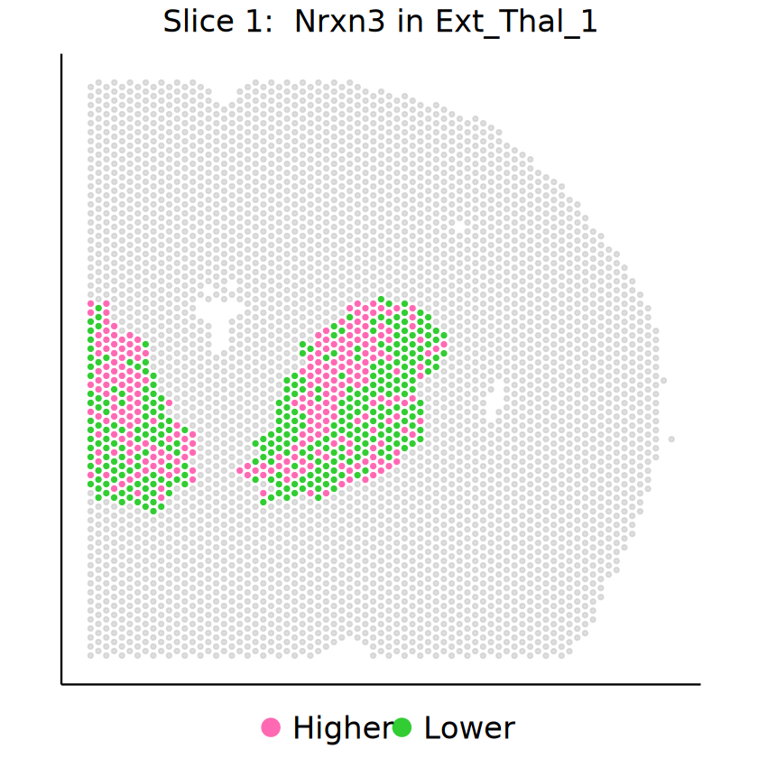
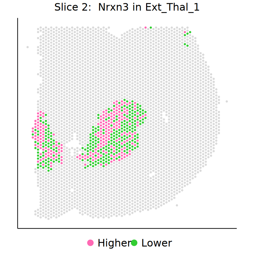
demo_genes <- c("Pcp4", "Nrxn3")
demo_genes_df <- pvalues_plot_df[(pvalues_plot_df$gene %in% demo_genes) & (pvalues_plot_df$case == "Real case"), ]
[21]:
expected_minus_log10p_lab <- expression(paste("Expected -log"[10], plain(P)))
observed_minus_log10p_lab <- expression(paste("Observed -log"[10], plain(P)))
p <- ggplot(data = pvalues_plot_df, aes(x = minus_log10p_theoretical, y = minus_log10p)) +
geom_point(aes(color = case), size = 5, alpha = 0.5) +
geom_abline(intercept = 0, slope = 1, linetype = "dashed", linewidth = 2) +
geom_point(data = demo_genes_df, color = "dodgerblue", size = 5, alpha = 1) +
ggrepel::geom_text_repel(
data = demo_genes_df, aes(label = gene),
color = "dodgerblue", size = 5, fontface = "bold.italic",
direction = "y", vjust = 0, hjust = 1, point.size = 5
) +
labs(
title = celltype,
x = expected_minus_log10p_lab, y = observed_minus_log10p_lab
) +
facet_wrap(. ~ slice, nrow = 1) +
theme_classic() +
theme(
text = element_text(family = "Helvetica", size = 16),
plot.title = element_text(size = 20, hjust = 0.5),
axis.title = element_text(size = 20),
axis.text.x = element_text(size = 18),
axis.text.y = element_text(size = 18),
strip.text = element_text(size = 20),
legend.title = element_blank(),
legend.text = element_text(size = 20),
legend.position = "bottom"
)
ggsave(
filename = file.path(RESULT_PATH, paste0("pvalue_qqplot_", celltype, ".pdf")),
plot = p, width = 6, height = 5
)
p

[22]:
for (gene in demo_genes) {
p1 <- mcubePlotExprCellTypeBinary(
mcube_object_1,
celltype = celltype, gene = gene, background = TRUE,
opacity_target = 1, opacity_background = 0.5,
) + guides(color = guide_legend(override.aes = list(size = 5))) +
labs(title = bquote("Slice 1: "~ italic(.(gene)) ~ "in" ~ .(celltype))) +
theme(
text = element_text(family = "Helvetica", size = 16),
plot.title = element_text(size = 20, hjust = 0.5),
axis.text.x = element_blank(),
axis.text.y = element_blank(),
axis.ticks = element_blank(),
legend.title = element_blank(),
legend.text = element_text(size = 20),
legend.position = "bottom"
)
ggsave(
filename = file.path(RESULT_PATH, paste0(celltype, "_", gene, "_slice_1", ".pdf")),
plot = p1, width = 4, height = 5
)
p2 <- mcubePlotExprCellTypeBinary(
mcube_object_2,
celltype = celltype, gene = gene, background = TRUE,
opacity_target = 1, opacity_background = 0.5,
) + guides(color = guide_legend(override.aes = list(size = 5))) +
labs(title = bquote("Slice 2: "~ italic(.(gene)) ~ "in" ~ .(celltype))) +
theme(
text = element_text(family = "Helvetica", size = 16),
plot.title = element_text(size = 20, hjust = 0.5),
axis.text.x = element_blank(),
axis.text.y = element_blank(),
axis.ticks = element_blank(),
legend.title = element_blank(),
legend.text = element_text(size = 20),
legend.position = "bottom"
)
ggsave(
filename = file.path(RESULT_PATH, paste0(celltype, "_", gene, "_slice_2", ".pdf")),
plot = p2, width = 4, height = 5
)
}
p1
p2
Cell type Inh_1
[23]:
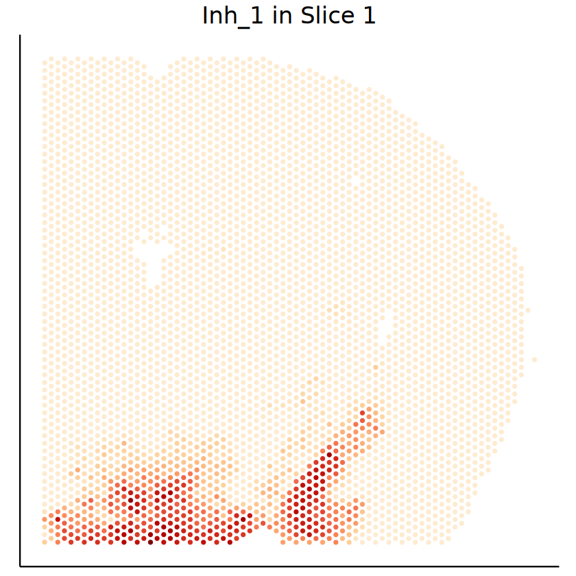
celltype <- "Inh_1"
p1 <- mcubePlotPropCellType(mcube_object_1@proportions, mcube_object_1@coordinates, celltype) +
labs(title = paste(celltype, "in Slice 1")) +
theme(
text = element_text(size = 1, hjust = 0.5),
plot.title = element_text(size = 20, hjust = 0.5),
axis.title = element_blank(),
axis.text.x = element_blank(),
axis.text.y = element_blank(),
axis.ticks = element_blank(),
legend.position = "none"
)
ggsave(
filename = file.path(RESULT_PATH, paste0("proportion_", celltype, "_slice_1", ".pdf")),
plot = p1, width = 4, height = 4
)
p2 <- mcubePlotPropCellType(mcube_object_2@proportions, mcube_object_2@coordinates, celltype) +
labs(title = paste(celltype, "in Slice 2")) +
theme(
text = element_text(size = 1, hjust = 0.5),
plot.title = element_text(size = 20, hjust = 0.5),
axis.title = element_blank(),
axis.text.x = element_blank(),
axis.text.y = element_blank(),
axis.ticks = element_blank(),
legend.position = "none"
)
ggsave(
filename = file.path(RESULT_PATH, paste0("proportion_", celltype, "_slice_2", ".pdf")),
plot = p2, width = 4, height = 4
)
p1
p2

[24]:
minus_log10p_max <- 5
pvalues_plot_df <- rbind(
data.frame(
mcubeQQPlotDF(pvalues_null_1[[celltype]], minus_log10p_max = 5),
slice = "Slice 1",
case = "Negative control"
),
data.frame(
mcubeQQPlotDF(pvalues_null_2[[celltype]], minus_log10p_max = 5),
slice = "Slice 2",
case = "Negative control"
),
data.frame(
mcubeQQPlotDF(mcube_object_1@pvalues[[celltype]], minus_log10p_max = 5),
slice = "Slice 1",
case = "Real case"
),
data.frame(
mcubeQQPlotDF(mcube_object_2@pvalues[[celltype]], minus_log10p_max = 5),
slice = "Slice 2",
case = "Real case"
)
)
pvalues_plot_df$case <- factor(pvalues_plot_df$case, levels = c("Real case", "Negative control"))
head(pvalues_plot_df[(pvalues_plot_df$slice == "Slice 1") & (pvalues_plot_df$case == "Real case"), ])
head(pvalues_plot_df[(pvalues_plot_df$slice == "Slice 2") & (pvalues_plot_df$case == "Real case"), ])
| gene | pvalue | pvalue_theoretical | minus_log10p | minus_log10p_theoretical | slice | case | |
|---|---|---|---|---|---|---|---|
| <chr> | <dbl> | <dbl> | <dbl> | <dbl> | <chr> | <fct> | |
| 2053 | Pmch | 3.432879e-227 | 0.0004975124 | 5 | 3.303196 | Slice 1 | Real case |
| 2054 | Gal | 2.052655e-80 | 0.0014925373 | 5 | 2.826075 | Slice 1 | Real case |
| 2055 | Vsnl1 | 1.337647e-64 | 0.0024875622 | 5 | 2.604226 | Slice 1 | Real case |
| 2056 | Rasgrf2 | 1.621062e-58 | 0.0034825871 | 5 | 2.458098 | Slice 1 | Real case |
| 2057 | Dlk1 | 1.103690e-55 | 0.0044776119 | 5 | 2.348954 | Slice 1 | Real case |
| 2058 | Camk2d | 2.890414e-55 | 0.0054726368 | 5 | 2.261803 | Slice 1 | Real case |
| gene | pvalue | pvalue_theoretical | minus_log10p | minus_log10p_theoretical | slice | case | |
|---|---|---|---|---|---|---|---|
| <chr> | <dbl> | <dbl> | <dbl> | <dbl> | <chr> | <fct> | |
| 3058 | Pmch | 1.089767e-170 | 0.0004775549 | 5 | 3.320977 | Slice 2 | Real case |
| 3059 | Gal | 1.707627e-68 | 0.0014326648 | 5 | 2.843855 | Slice 2 | Real case |
| 3060 | Vsnl1 | 3.919878e-51 | 0.0023877746 | 5 | 2.622007 | Slice 2 | Real case |
| 3061 | Dlk1 | 1.704307e-44 | 0.0033428844 | 5 | 2.475879 | Slice 2 | Real case |
| 3062 | Atp2b4 | 4.548976e-43 | 0.0042979943 | 5 | 2.366734 | Slice 2 | Real case |
| 3063 | Peg3 | 3.590220e-41 | 0.0052531041 | 5 | 2.279584 | Slice 2 | Real case |
[25]:
# demo_genes <- c("Pmch", "Gal") # Camk2d, Slc32a1, Unc13c, Nsf
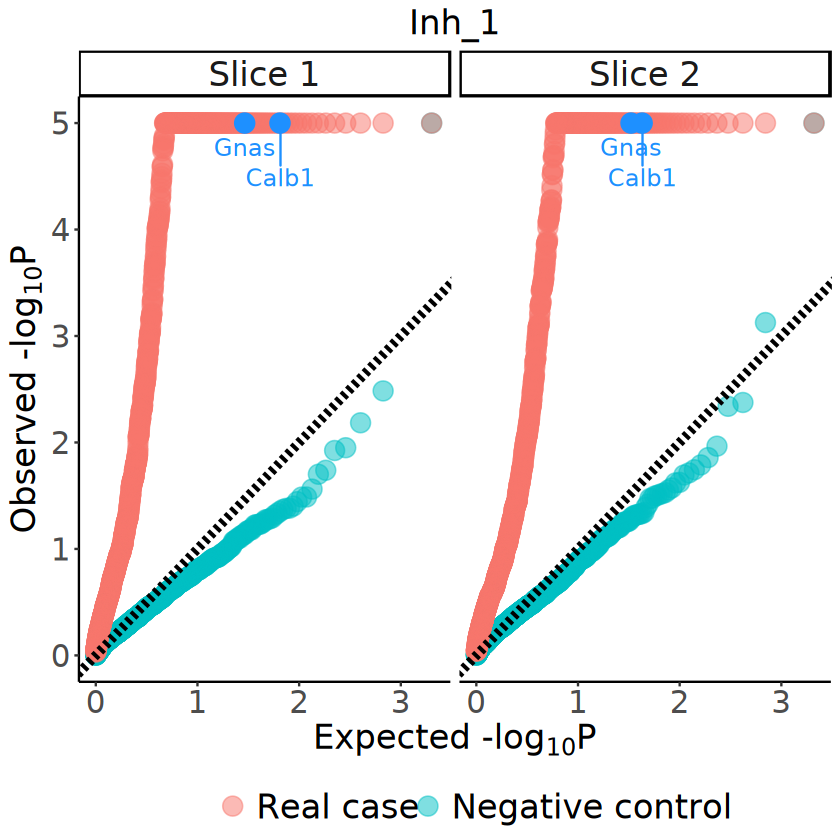
demo_genes <-c("Calb1", "Gnas")
demo_genes_df <- pvalues_plot_df[(pvalues_plot_df$gene %in% demo_genes) & (pvalues_plot_df$case == "Real case"), ]
[26]:
p <- ggplot(data = pvalues_plot_df, aes(x = minus_log10p_theoretical, y = minus_log10p)) +
geom_point(aes(color = case), size = 5, alpha = 0.5) +
geom_abline(intercept = 0, slope = 1, linetype = "dashed", linewidth = 2) +
geom_point(data = demo_genes_df, color = "dodgerblue", size = 5, alpha = 1) +
ggrepel::geom_text_repel(
data = demo_genes_df, aes(label = gene),
color = "dodgerblue", size = 5, fontface = "bold.italic",
direction = "y", vjust = -0.5, hjust = 0.5, point.size = 5
) +
labs(
title = celltype,
x = expected_minus_log10p_lab, y = observed_minus_log10p_lab
) +
facet_wrap(. ~ slice, nrow = 1) +
theme_classic() +
theme(
text = element_text(family = "Helvetica", size = 16),
plot.title = element_text(size = 20, hjust = 0.5),
axis.title = element_text(size = 20),
axis.text.x = element_text(size = 18),
axis.text.y = element_text(size = 18),
strip.text = element_text(size = 20),
legend.title = element_blank(),
legend.text = element_text(size = 20),
legend.position = "bottom"
)
ggsave(
filename = file.path(RESULT_PATH, paste0("pvalue_qqplot_", celltype, ".pdf")),
plot = p, width = 6, height = 5
)
p
[27]:
for (gene in demo_genes) {
p1 <- mcubePlotExprCellTypeBinary(
mcube_object_1,
celltype = celltype, gene = gene, background = TRUE,
opacity_target = 1, opacity_background = 0.5,
) + guides(color = guide_legend(override.aes = list(size = 5))) +
labs(title = bquote("Slice 1: "~ italic(.(gene)) ~ "in" ~ .(celltype))) +
theme(
text = element_text(family = "Helvetica", size = 16),
plot.title = element_text(size = 20, hjust = 0.5),
axis.text.x = element_blank(),
axis.text.y = element_blank(),
axis.ticks = element_blank(),
legend.title = element_blank(),
legend.text = element_text(size = 20),
legend.position = "bottom"
)
ggsave(
filename = file.path(RESULT_PATH, paste0(celltype, "_", gene, "_slice_1", ".pdf")),
plot = p1, width = 4, height = 5
)
p2 <- mcubePlotExprCellTypeBinary(
mcube_object_2,
celltype = celltype, gene = gene, background = TRUE,
opacity_target = 1, opacity_background = 0.5,
) + guides(color = guide_legend(override.aes = list(size = 5))) +
labs(title = bquote("Slice 2: "~ italic(.(gene)) ~ "in" ~ .(celltype))) +
theme(
text = element_text(family = "Helvetica", size = 16),
plot.title = element_text(size = 20, hjust = 0.5),
axis.text.x = element_blank(),
axis.text.y = element_blank(),
axis.ticks = element_blank(),
legend.title = element_blank(),
legend.text = element_text(size = 20),
legend.position = "bottom"
)
ggsave(
filename = file.path(RESULT_PATH, paste0(celltype, "_", gene, "_slice_2", ".pdf")),
plot = p2, width = 4, height = 5
)
}
p1
p2


[28]:
rm(mcube_object_1, mcube_object_2, pvalues_null_1, pvalues_null_2)
3D adult mouse brain model constructed from Spatial Transcriptomics dataset
[29]:
n_slices <- 35
slice_idx_seq <- c(1:n_slices)
reference_ST <- data.matrix(
read.csv(file.path(DATA_PATH, "ST_3D", "reference_ST.csv"),
header = TRUE, row.names = 1, check.names = FALSE
)
)
dim(reference_ST)
num_celltypes <- nrow(reference_ST)
proportions_ST <- matrix(, nrow = 0, ncol = num_celltypes)
batch_id <- vector("character")
for(slice_idx in slice_idx_seq){
proportions_i <- as.matrix(read.csv(
file.path(
DATA_PATH, "ST_3D",
paste0("prop_slice", slice_idx - 1, ".csv")
),
header = TRUE, row.names = 1, check.names = FALSE
))
proportions_ST <- rbind(proportions_ST, proportions_i)
batch_id <- c(batch_id, rep(paste0("slice", slice_idx - 1), nrow(proportions_i)))
}
dim(proportions_ST)
num_spots <- nrow(proportions_ST)
spots <- rownames(proportions_ST)
names(batch_id) <- spots
counts <- as.data.frame(readr::read_csv(
file.path(DATA_PATH, "ST_3D", "counts.csv")
))
rownames(counts) <- counts[, 1]
counts[, 1] <- NULL
counts <- counts[spots, ]
counts <- data.matrix(counts)
dim(counts)
coordinates <- as.matrix(read.csv(
file.path(DATA_PATH, "ST_3D", "3D_coordinates.csv"),
header = TRUE, row.names = 1, check.names = FALSE
))
shuffle_idx <- sample(1:nrow(coordinates), nrow(coordinates))
write.csv(shuffle_idx, file = file.path(DATA_PATH, "ST_3D", "shuffle_idx.csv"), row.names = FALSE)
shuffle_idx <- read.csv(file.path(DATA_PATH, "ST_3D", "shuffle_idx.csv"), header = TRUE)[, 1]
length(unique(shuffle_idx))
coordinates_shuffle <- coordinates[shuffle_idx, ]
rownames(coordinates_shuffle) <- rownames(coordinates)
write.csv(coordinates_shuffle, file = file.path(DATA_PATH, "ST_3D", "3D_coordinates_shuffle.csv"))
coordinates_shuffle <- as.matrix(read.csv(
file.path(DATA_PATH, "ST_3D", "3D_coordinates_shuffle.csv"),
header = TRUE, row.names = 1, check.names = FALSE
))
coordinates <- coordinates[spots, ]
coordinates_shuffle <- coordinates_shuffle[spots, ]
dim(coordinates)
dim(coordinates_shuffle)
spot_effects_ST <- data.matrix(read.csv(
file.path(DATA_PATH, "ST_3D", "spot_effects_ST.csv"),
header = TRUE, row.names = 1, check.names = FALSE
))[spots, 1]
platform_effects_ST <- data.matrix(read.csv(
file.path(DATA_PATH, "ST_3D", "platform_effects_ST.csv"),
header = TRUE, row.names = 1, check.names = FALSE
))
library_sizes_ST <- data.matrix(read.csv(
file.path(DATA_PATH, "ST_3D", "library_sizes_ST.csv"),
header = TRUE, row.names = 1, check.names = FALSE
))[spots, 1]
- 59
- 6227
- 17086
- 59
New names:
• `` -> `...1`
Rows: 17086 Columns: 6228
── Column specification ────────────────────────────────────────────────────────
Delimiter: ","
chr (1): ...1
dbl (6227): A230001M10Rik, A230006K03Rik, A230009B12Rik, A230065N10Rik, A230...
ℹ Use `spec()` to retrieve the full column specification for this data.
ℹ Specify the column types or set `show_col_types = FALSE` to quiet this message.
- 17086
- 6227
17086
- 17086
- 3
- 17086
- 3
[30]:
# Real case
mcube_object_3D <- createMCube(
counts = counts, coordinates = coordinates,
proportions = proportions_ST, library_sizes = library_sizes_ST,
covariates = NULL, batch_id = batch_id,
reference = reference_ST,
spot_effects = spot_effects_ST, platform_effects = platform_effects_ST,
project = "mouse_brain_3D"
)
mcube_object_3D <- mcubeFitNull(
mcube_object_3D,
num_workers = 70, num_threads = 1
)
mcube_object_3D <- mcubeTest(
mcube_object_3D,
num_workers = 70, num_threads = 1, shared_memory = TRUE
)
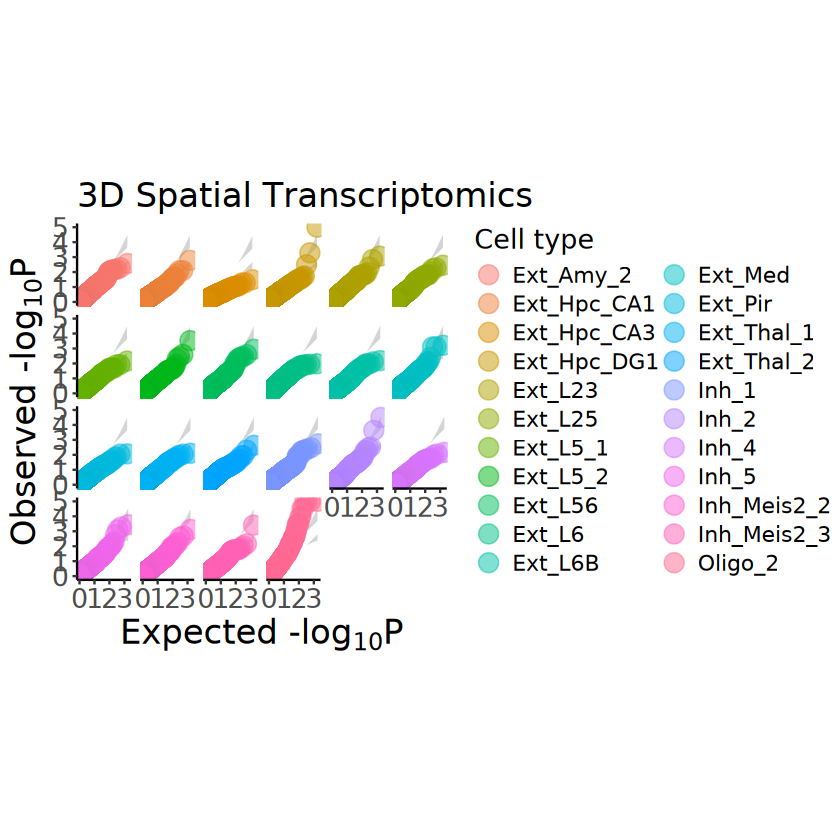
p <- mcubePlotPvalues(mcube_object_3D@pvalues, "combined_pvalue", nrow = 4)
p <- p +
labs(title = "3D Spatial Transcriptomics") +
theme(
text = element_text(size = 16),
plot.title = element_text(size = 20),
axis.title = element_text(size = 20),
axis.text.x = element_text(size = 16),
axis.text.y = element_text(size = 16)
)
ggsave(
filename = file.path(
RESULT_PATH, "ST_3D",
paste0("pvalue_qqplot.png")
),
plot = p, width = 12, height = 12
)
p
Select high-abundance cell types to analyze with proportion_threshold = 0.1 and celltype_threshold = 100.
mcubeFilterCellTypes: Cell type(s) Ext_Amy_2, Ext_Hpc_CA1, Ext_Hpc_CA3, Ext_Hpc_DG1, Ext_L23, Ext_L25, Ext_L56, Ext_L5_1, Ext_L5_2, Ext_L6, Ext_L6B, Ext_Med, Ext_Pir, Ext_Thal_1, Ext_Thal_2, Inh_1, Inh_2, Inh_4, Inh_5, Inh_Meis2_2, Inh_Meis2_3, Oligo_2 pass the threshold.
Cell type(s) Astro_AMY, Astro_AMY_CTX, Astro_CTX, Astro_HPC, Astro_HYPO, Astro_STR, Astro_THAL_hab, Astro_THAL_lat, Astro_THAL_med, Astro_WM, Endo, Ext_Amy_1, Ext_ClauPyr, Ext_Hpc_CA2, Ext_Hpc_DG2, Ext_L5_3, Ext_Unk_1, Ext_Unk_2, Ext_Unk_3, Inh_3, Inh_6, Inh_Lamp5, Inh_Meis2_1, Inh_Meis2_4, Inh_Pvalb, Inh_Sst, Inh_Vip, LowQ_1, LowQ_2, Micro, Nb_1, Nb_2, OPC_1, OPC_2, Oligo_1, Unk_1, Unk_2 has/have less than the minimum celltype_threshold = 100 with proportion_threshold = 0.1.
To include the above cell type(s), please reduce celltype_threshold or proportion_threshold.
Cell type(s) Ext_Amy_2, Ext_Hpc_CA1, Ext_Hpc_CA3, Ext_Hpc_DG1, Ext_L23, Ext_L25, Ext_L56, Ext_L5_1, Ext_L5_2, Ext_L6, Ext_L6B, Ext_Med, Ext_Pir, Ext_Thal_1, Ext_Thal_2, Inh_1, Inh_2, Inh_4, Inh_5, Inh_Meis2_2, Inh_Meis2_3, Oligo_2 will be analyzed.
Filter out lowly-expressed genes with gene_threshold = 5e-05.
mcubeFilterGenes: 2841 genes pass the threshold.
Select highly-expressed genes to analyze for each specific cell type with reference_threshold = 0.5.
mcubeFilterGenesCellType: Select 1091 genes to analyze for Ext_Amy_2.
mcubeFilterGenesCellType: Select 926 genes to analyze for Ext_Hpc_CA1.
mcubeFilterGenesCellType: Select 850 genes to analyze for Ext_Hpc_CA3.
mcubeFilterGenesCellType: Select 1113 genes to analyze for Ext_Hpc_DG1.
mcubeFilterGenesCellType: Select 1000 genes to analyze for Ext_L23.
mcubeFilterGenesCellType: Select 1049 genes to analyze for Ext_L25.
mcubeFilterGenesCellType: Select 1089 genes to analyze for Ext_L56.
mcubeFilterGenesCellType: Select 1000 genes to analyze for Ext_L5_1.
mcubeFilterGenesCellType: Select 982 genes to analyze for Ext_L5_2.
mcubeFilterGenesCellType: Select 1061 genes to analyze for Ext_L6.
mcubeFilterGenesCellType: Select 1126 genes to analyze for Ext_L6B.
mcubeFilterGenesCellType: Select 1073 genes to analyze for Ext_Med.
mcubeFilterGenesCellType: Select 1060 genes to analyze for Ext_Pir.
mcubeFilterGenesCellType: Select 1032 genes to analyze for Ext_Thal_1.
mcubeFilterGenesCellType: Select 1125 genes to analyze for Ext_Thal_2.
mcubeFilterGenesCellType: Select 1320 genes to analyze for Inh_1.
mcubeFilterGenesCellType: Select 1254 genes to analyze for Inh_2.
mcubeFilterGenesCellType: Select 1331 genes to analyze for Inh_4.
mcubeFilterGenesCellType: Select 1235 genes to analyze for Inh_5.
mcubeFilterGenesCellType: Select 1087 genes to analyze for Inh_Meis2_2.
mcubeFilterGenesCellType: Select 1062 genes to analyze for Inh_Meis2_3.
mcubeFilterGenesCellType: Select 1246 genes to analyze for Oligo_2.
Preprocessed data description: 17065 spots and 59 cell types in total. 16307 spots, 2840 genes, and 22 cell type(s) to analyze.
Number of physical cores: 72.
Number of workers: 70.
Number of thread(s) on BLAS per worker: 1.
mcubeKernel: length_scale is set as 0.15924412901695 for the Gaussian kernel.
mcubeKernel: length_scale is set as 0.225205206984061 for the Gaussian kernel.
mcubeKernel: length_scale is set as 0.15924412901695 for the Gaussian_transformed kernel.
mcubeKernel: length_scale is set as 0.225205206984061 for the Gaussian_transformed kernel.
Number of physical cores: 72.
Number of workers: 70.
Number of thread(s) on BLAS per worker: 1.

[31]:
saveRDS(
mcube_object_3D,
file = file.path(
RESULT_PATH, "ST_3D",
paste0("mcube", ".rds")
)
)
# mcube_object_3D <- readRDS(
# file = file.path(
# RESULT_PATH, "ST_3D",
# paste0("mcube", ".rds")
# )
# )
[32]:
# Negative control
mcube_object_null_3D <- mcube_object_3D
mcube_object_null_3D@coordinates <- as.matrix(coordinates_shuffle)
mcube_object_null_3D <- mcubeTest(
mcube_object_null_3D,
num_workers = 70, num_threads = 1, shared_memory = TRUE
)
pvalues_null_3D <- mcube_object_null_3D@pvalues
rm(mcube_object_null_3D)
p <- mcubePlotPvalues(pvalues_null_3D, "combined_pvalue", nrow = 4, under_null = TRUE)
p <- p +
labs(title = "3D Spatial Transcriptomics") +
theme(
text = element_text(size = 16),
plot.title = element_text(size = 20),
axis.title = element_text(size = 20),
axis.text.x = element_text(size = 16),
axis.text.y = element_text(size = 16)
)
ggsave(
filename = file.path(
RESULT_PATH, "ST_3D",
paste0("p_value_qqplot_null.png")),
plot = p, width = 12, height = 7
)
p
mcubeKernel: length_scale is set as 0.158383855293133 for the Gaussian kernel.
mcubeKernel: length_scale is set as 0.223988596216487 for the Gaussian kernel.
mcubeKernel: length_scale is set as 0.158383855293133 for the Gaussian_transformed kernel.
mcubeKernel: length_scale is set as 0.223988596216487 for the Gaussian_transformed kernel.
Number of physical cores: 72.
Number of workers: 70.
Number of thread(s) on BLAS per worker: 1.
[33]:
saveRDS(
pvalues_null_3D,
file = file.path(
RESULT_PATH, "ST_3D",
paste0("mcube_pvalues_null", ".rds")
)
)
# pvalues_null_3D <- readRDS(
# file = file.path(
# RESULT_PATH, "ST_3D",
# paste0("mcube_pvalues_null", ".rds")
# )
# )
Visualization
[34]:
mcube_object_3D <- readRDS(
file = file.path(
RESULT_PATH, "ST_3D",
paste0("mcube", ".rds")
)
)
pvalues_null_3D <- readRDS(
file = file.path(
RESULT_PATH, "ST_3D",
paste0("mcube_pvalues_null", ".rds")
)
)
[35]:
minus_log10p_max <- 5
demo_celltypes <- c("Ext_Thal_1", "Inh_1")
pvalues_plot_df <- data.frame()
for (celltype in demo_celltypes) {
pvalues_plot_df <- rbind(
pvalues_plot_df,
data.frame(
mcubeQQPlotDF(pvalues_null_3D[[celltype]], minus_log10p_max = 5),
case = "Negative control",
celltype = celltype
),
data.frame(
mcubeQQPlotDF(mcube_object_3D@pvalues[[celltype]], minus_log10p_max = 5),
case = "Real case",
celltype = celltype
)
)
}
pvalues_plot_df$case <- factor(pvalues_plot_df$case, levels = c("Real case", "Negative control"))
head(pvalues_plot_df[pvalues_plot_df$case == "Real case", ])
| gene | pvalue | pvalue_theoretical | minus_log10p | minus_log10p_theoretical | case | celltype | |
|---|---|---|---|---|---|---|---|
| <chr> | <dbl> | <dbl> | <dbl> | <dbl> | <fct> | <chr> | |
| 775 | Nsmf | 1.045641e-63 | 0.0006459948 | 5 | 3.189771 | Real case | Ext_Thal_1 |
| 776 | Pcp4 | 3.496110e-62 | 0.0019379845 | 5 | 2.712650 | Real case | Ext_Thal_1 |
| 777 | Cplx1 | 2.413101e-43 | 0.0032299742 | 5 | 2.490801 | Real case | Ext_Thal_1 |
| 778 | Atp2a2 | 7.523337e-36 | 0.0045219638 | 5 | 2.344673 | Real case | Ext_Thal_1 |
| 779 | Gprasp1 | 6.810823e-31 | 0.0058139535 | 5 | 2.235528 | Real case | Ext_Thal_1 |
| 780 | Rora | 6.613392e-30 | 0.0071059432 | 5 | 2.148378 | Real case | Ext_Thal_1 |
[36]:
demo_genes <- list(
Ext_Thal_1 = c("Pcp4", "Nrxn3"),
Inh_1 = c("Calb1", "Gnas")
)
demo_genes_df <- rbind(
pvalues_plot_df[
(pvalues_plot_df$celltype == demo_celltypes[1]) &
(pvalues_plot_df$gene %in% demo_genes[[1]]) &
(pvalues_plot_df$case == "Real case"),
],
pvalues_plot_df[
(pvalues_plot_df$celltype == demo_celltypes[2]) &
(pvalues_plot_df$gene %in% demo_genes[[2]]) &
(pvalues_plot_df$case == "Real case"),
]
)
demo_genes_df
| gene | pvalue | pvalue_theoretical | minus_log10p | minus_log10p_theoretical | case | celltype | |
|---|---|---|---|---|---|---|---|
| <chr> | <dbl> | <dbl> | <dbl> | <dbl> | <fct> | <chr> | |
| 776 | Pcp4 | 3.496110e-62 | 0.0019379845 | 5 | 2.712650 | Real case | Ext_Thal_1 |
| 787 | Nrxn3 | 2.314395e-22 | 0.0161498708 | 5 | 1.791831 | Real case | Ext_Thal_1 |
| 2488 | Calb1 | 1.305533e-57 | 0.0005324814 | 5 | 3.273696 | Real case | Inh_1 |
| 2493 | Gnas | 6.143010e-30 | 0.0058572950 | 5 | 2.232303 | Real case | Inh_1 |
[37]:
expected_minus_log10p_lab <- expression(paste("Expected -log"[10], plain(P)))
observed_minus_log10p_lab <- expression(paste("Observed -log"[10], plain(P)))
p <- ggplot(data = pvalues_plot_df, aes(x = minus_log10p_theoretical, y = minus_log10p)) +
geom_point(aes(color = case), size = 5, alpha = 0.5) +
geom_abline(intercept = 0, slope = 1, linetype = "dashed", linewidth = 2) +
geom_point(data = demo_genes_df, color = "dodgerblue", size = 5, alpha = 1) +
ggrepel::geom_text_repel(
data = demo_genes_df, aes(label = gene),
color = "dodgerblue", size = 5, fontface = "bold.italic",
direction = "y", vjust = 0, hjust = 1, point.size = 5
) +
labs(
title = "3D model reconstructed from the ST data",
x = expected_minus_log10p_lab, y = observed_minus_log10p_lab
) +
facet_wrap(. ~ celltype, nrow = 1) +
theme_classic() +
theme(
text = element_text(family = "Helvetica", size = 16),
plot.title = element_text(size = 20, hjust = 0.5),
axis.title = element_text(size = 20),
axis.text.x = element_text(size = 18),
axis.text.y = element_text(size = 18),
strip.text = element_text(size = 20),
legend.title = element_blank(),
legend.text = element_text(size = 20),
legend.position = "bottom"
)
ggsave(
filename = file.path(RESULT_PATH, paste0("pvalue_qqplot_3D", ".pdf")),
plot = p, width = 6, height = 5
)
p

[38]:
# # For saving the plotly object as a static image with `kaleido`
# install.packages('reticulate')
# reticulate::install_miniconda()
# reticulate::conda_install('r-reticulate', 'python-kaleido')
# reticulate::conda_install('r-reticulate', 'plotly', channel = 'plotly')
# reticulate::use_miniconda('r-reticulate')
[39]:
celltype <- demo_celltypes[1]
p <- mcubePlotPropCellType3D(
mcube_object_3D@proportions, mcube_object_3D@coordinates, celltype,
spot_size = 1.5, opacity_background = 0.05,
plotly_eye = list(x = 1.8, y = 0.5, z = 1.8)
)
plotly::save_image(
p, file.path(RESULT_PATH, paste0("proportion_", celltype, "_3D", ".pdf")),
width = 500, height = 500, scale = 5
)
p
[40]:
gene <- demo_genes[[demo_celltypes[1]]][1]
p <- mcubePlotExprCellType3D(
mcube_object_3D, celltype, gene,
spot_size = 1.5, opacity_target = 0.7, opacity_background = 0.05,
plotly_eye = list(x = 1.8, y = 0.5, z = 1.8)
)
plotly::save_image(
p, file.path(RESULT_PATH, paste0(celltype, "_", gene, "_3D", ".pdf")),
width = 500, height = 500, scale = 5
)
gene <- demo_genes[[demo_celltypes[1]]][2]
p <- mcubePlotExprCellType3D(
mcube_object_3D, celltype, gene,
spot_size = 1.5, opacity_target = 0.7, opacity_background = 0.05,
plotly_eye = list(x = 1.8, y = 0.5, z = 1.8)
)
plotly::save_image(
p, file.path(RESULT_PATH, paste0(celltype, "_", gene, "_3D", ".pdf")),
width = 500, height = 500, scale = 5
)
p
[41]:
celltype <- demo_celltypes[2]
p <- mcubePlotPropCellType3D(
mcube_object_3D@proportions, mcube_object_3D@coordinates, celltype,
spot_size = 1.5, opacity_background = 0.05,
plotly_eye = list(x = -0.8, y = -1.2, z = 1.6)
)
plotly::save_image(
p, file.path(RESULT_PATH, paste0("proportion_", celltype, "_3D", ".pdf")),
width = 500, height = 500, scale = 5
)
p
[42]:
celltype <- demo_celltypes[2]
gene <- demo_genes[[demo_celltypes[2]]][1]
p <- mcubePlotExprCellType3D(
mcube_object_3D, celltype, gene,
spot_size = 1.5, opacity_target = 0.7, opacity_background = 0.05,
plotly_eye = list(x = -0.8, y = -1.2, z = 1.6)
)
plotly::save_image(
p, file.path(RESULT_PATH, paste0(celltype, "_", gene, "_3D", ".pdf")),
width = 500, height = 500, scale = 5
)
gene <- demo_genes[[demo_celltypes[2]]][2]
p <- mcubePlotExprCellType3D(
mcube_object_3D, celltype, gene,
spot_size = 1.5, opacity_target = 0.7, opacity_background = 0.05,
plotly_eye = list(x = -0.8, y = -1.2, z = 1.6)
)
plotly::save_image(
p, file.path(RESULT_PATH, paste0(celltype, "_", gene, "_3D", ".pdf")),
width = 500, height = 500, scale = 5
)
p
[43]:
# For 3D visualizations in the Allen Mouse Brain Common Coordinate Framework (CCFv3) using rgl and misc3d
demo_celltype_gene_pairs <- c(
paste0(demo_celltypes[1], "_", demo_genes[[1]]),
paste0(demo_celltypes[2], "_", demo_genes[[2]])
)
plot3D_data <- list(
proportions = mcube_object_3D@proportions,
coordinates = mcube_object_3D@coordinates,
null_models = mcube_object_3D@null_models[demo_celltype_gene_pairs]
)
saveRDS(
plot3D_data,
file = file.path(
RESULT_PATH, "ST_3D",
paste0("plot3D_data", ".rds")
)
)
[ ]: