Sentivity and replicability analysis of `MCube`

We first analyze the senesitivity of MCube to cell type deconvolution using the Visium data. Specifically, we compare the results from MCube when integrting the estimated cell type proportions from two different methods (RCTD and STitch3D). To examine whether the results are replicable, we then compare the results from MCube on the two slices of the Visium data.

[1]:

set.seed(20250428)

library(Matrix)
library(spacexr)
library(MCube)

library(dplyr)
library(ggplot2)


Attaching package: ‘dplyr’


The following objects are masked from ‘package:stats’:

    filter, lag


The following objects are masked from ‘package:base’:

    intersect, setdiff, setequal, union

[2]:

# RAW_DATA_PATH <- "/import/home/share/zw/data/mouse_brain"
RAW_DATA_PATH <- "/import/home/share/zw/pql/data/mouse_brain"
DATA_PATH <- "/import/home/share/zw/pql/data/mouse_brain/reliability"
RESULT_PATH <- "/import/home/share/zw/pql/results/mouse_brain/reliability"

if (!dir.exists(file.path(DATA_PATH, "visium_1"))) {
    dir.create(file.path(DATA_PATH, "visium_1"), recursive = TRUE)
}
if (!dir.exists(file.path(DATA_PATH, "visium_2"))) {
    dir.create(file.path(DATA_PATH, "visium_2"), recursive = TRUE)
}
if (!dir.exists(file.path(RESULT_PATH, "visium_1"))) {
    dir.create(file.path(RESULT_PATH, "visium_1"), recursive = TRUE)
}
if (!dir.exists(file.path(RESULT_PATH, "visium_2"))) {
    dir.create(file.path(RESULT_PATH, "visium_2"), recursive = TRUE)
}

[3]:

# scRNA-seq reference data
sc_counts <- as.data.frame(readr::read_csv(
    file.path(RAW_DATA_PATH, "visium_1", "sc_counts.csv")
))
rownames(sc_counts) <- sc_counts[, 1]
sc_counts[, 1] <- NULL
sc_counts <- as.matrix(sc_counts)
dim(sc_counts)

sc_labels <- as.matrix(read.csv(
    file.path(RAW_DATA_PATH, "visium_1", "sc_labels.csv"),
    header = TRUE, row.names = 1
))[, 1]
# Exclude cells with unknown or low quality labels
# ex_cells <- grep("Unk|LowQ", sc_labels)
ex_cells <- which(sc_labels == "Unk_1")
sc_labels <- sc_labels[-ex_cells]
sc_labels <- factor(sc_labels, levels = unique(sc_labels))

sc_counts <- sc_counts[-ex_cells, ]

reference <- Reference(t(sc_counts), sc_labels, rowSums(sc_counts))

New names:
• `` -> `...1`
Rows: 40532 Columns: 6416
── Column specification ────────────────────────────────────────────────────────
Delimiter: ","
chr    (1): ...1
dbl (6415): 0610040J01Rik, 0610043K17Rik, 1110002J07Rik, 1110004F10Rik, 1110...

ℹ Use `spec()` to retrieve the full column specification for this data.
ℹ Specify the column types or set `show_col_types = FALSE` to quiet this message.

40532
6415

Warning message in Reference(t(sc_counts), sc_labels, rowSums(sc_counts)):
“Reference: number of cells per cell type is 10819, larger than maximum allowable of 10000. Downsampling number of cells to: 10000”

Visium Slice 1

[4]:

counts <- as.data.frame(readr::read_csv(
    file.path(RAW_DATA_PATH, "visium_1", "counts.csv")
))
rownames(counts) <- counts[, 1]
counts[, 1] <- NULL
counts <- as.matrix(counts)
dim(counts)

coordinates <- as.data.frame(readr::read_csv(
    file.path(RAW_DATA_PATH, "visium_1", "3D_coordinates.csv")
))
rownames(coordinates) <- coordinates[, 1]
coordinates[, c(1, 4)] <- NULL
coordinates <- as.matrix(coordinates)
dim(coordinates)

puck <- SpatialRNA(as.data.frame(coordinates), t(counts), rowSums(counts))

New names:
• `` -> `...1`
Rows: 4168 Columns: 6416
── Column specification ────────────────────────────────────────────────────────
Delimiter: ","
chr    (1): ...1
dbl (6415): 0610040J01Rik, 0610043K17Rik, 1110002J07Rik, 1110004F10Rik, 1110...

ℹ Use `spec()` to retrieve the full column specification for this data.
ℹ Specify the column types or set `show_col_types = FALSE` to quiet this message.

4168
6415

New names:
• `` -> `...1`
Rows: 4168 Columns: 4
── Column specification ────────────────────────────────────────────────────────
Delimiter: ","
chr (1): ...1
dbl (3): x, y, z

ℹ Use `spec()` to retrieve the full column specification for this data.
ℹ Specify the column types or set `show_col_types = FALSE` to quiet this message.

4168
2

Integrating with `RCTD`

Cell type deconvolution

[5]:

myRCTD <- create.RCTD(
    puck, reference,
    CELL_MIN_INSTANCE = 20, max_cores = 8
)
myRCTD <- run.RCTD(myRCTD, doublet_mode = "full")
saveRDS(myRCTD, file.path(RESULT_PATH, "visium_1", "myRCTD.rds"))

Begin: process_cell_type_info

process_cell_type_info: number of cells in reference: 38849

process_cell_type_info: number of genes in reference: 6415


       Ext_L23        Oligo_2 Astro_THAL_med        Inh_Sst          Inh_6
          1244          10000            405            640            467
      Ext_L5_3    Inh_Meis2_3          Micro       Ext_L5_2        Ext_Pir
           127            789           1218            166            954
     Astro_AMY          Inh_2          Inh_1      Inh_Pvalb      Inh_Lamp5
           498            839            573            804            331
       Ext_L25           Nb_2     Ext_Thal_1        Ext_L56      Ext_Unk_2
           922            203           1197           1422            205
     Ext_Unk_3          Inh_3      Ext_Amy_2     Ext_Thal_2       Ext_L5_1
           416            818            797            671            893
         OPC_1  Astro_AMY_CTX    Ext_Hpc_DG1     Astro_HYPO          Inh_4
          1015            279            554            451           1389
   Inh_Meis2_1    Ext_Hpc_DG2        Ext_Med    Inh_Meis2_2    Ext_Hpc_CA1
           363            915             70            602            671
       Ext_L6B      Astro_CTX      Ext_Amy_1       Astro_WM        Oligo_1
           356            443            519            220            613
     Astro_STR         Ext_L6 Astro_THAL_lat           Nb_1         LowQ_2
            81            568            332            225            265
       Inh_Vip      Astro_HPC    Ext_ClauPyr    Ext_Hpc_CA2          OPC_2
           545            261            272             48            300
         Inh_5    Ext_Hpc_CA3      Ext_Unk_1    Inh_Meis2_4          Unk_2
           118            232             90            193             85
Astro_THAL_hab         LowQ_1           Endo
            43            110             22

End: process_cell_type_info

create.RCTD: getting regression differentially expressed genes:

get_de_genes: Ext_L23 found DE genes: 112

get_de_genes: Oligo_2 found DE genes: 411

get_de_genes: Astro_THAL_med found DE genes: 353

get_de_genes: Inh_Sst found DE genes: 123

get_de_genes: Inh_6 found DE genes: 195

get_de_genes: Ext_L5_3 found DE genes: 134

get_de_genes: Inh_Meis2_3 found DE genes: 153

get_de_genes: Micro found DE genes: 647

get_de_genes: Ext_L5_2 found DE genes: 103

get_de_genes: Ext_Pir found DE genes: 69

get_de_genes: Astro_AMY found DE genes: 333

get_de_genes: Inh_2 found DE genes: 98

get_de_genes: Inh_1 found DE genes: 86

get_de_genes: Inh_Pvalb found DE genes: 131

get_de_genes: Inh_Lamp5 found DE genes: 166

get_de_genes: Ext_L25 found DE genes: 147

get_de_genes: Nb_2 found DE genes: 364

get_de_genes: Ext_Thal_1 found DE genes: 213

get_de_genes: Ext_L56 found DE genes: 157

get_de_genes: Ext_Unk_2 found DE genes: 151

get_de_genes: Ext_Unk_3 found DE genes: 151

get_de_genes: Inh_3 found DE genes: 88

get_de_genes: Ext_Amy_2 found DE genes: 74

get_de_genes: Ext_Thal_2 found DE genes: 151

get_de_genes: Ext_L5_1 found DE genes: 106

get_de_genes: OPC_1 found DE genes: 248

get_de_genes: Astro_AMY_CTX found DE genes: 348

get_de_genes: Ext_Hpc_DG1 found DE genes: 196

get_de_genes: Astro_HYPO found DE genes: 352

get_de_genes: Inh_4 found DE genes: 83

get_de_genes: Inh_Meis2_1 found DE genes: 127

get_de_genes: Ext_Hpc_DG2 found DE genes: 184

get_de_genes: Ext_Med found DE genes: 110

get_de_genes: Inh_Meis2_2 found DE genes: 157

get_de_genes: Ext_Hpc_CA1 found DE genes: 186

get_de_genes: Ext_L6B found DE genes: 155

get_de_genes: Astro_CTX found DE genes: 330

get_de_genes: Ext_Amy_1 found DE genes: 113

get_de_genes: Astro_WM found DE genes: 315

get_de_genes: Oligo_1 found DE genes: 358

get_de_genes: Astro_STR found DE genes: 343

get_de_genes: Ext_L6 found DE genes: 94

get_de_genes: Astro_THAL_lat found DE genes: 328

get_de_genes: Nb_1 found DE genes: 239

get_de_genes: LowQ_2 found DE genes: 158

get_de_genes: Inh_Vip found DE genes: 119

get_de_genes: Astro_HPC found DE genes: 337

get_de_genes: Ext_ClauPyr found DE genes: 134

get_de_genes: Ext_Hpc_CA2 found DE genes: 154

get_de_genes: OPC_2 found DE genes: 359

get_de_genes: Inh_5 found DE genes: 172

get_de_genes: Ext_Hpc_CA3 found DE genes: 135

get_de_genes: Ext_Unk_1 found DE genes: 182

get_de_genes: Inh_Meis2_4 found DE genes: 166

get_de_genes: Unk_2 found DE genes: 172

get_de_genes: Astro_THAL_hab found DE genes: 378

get_de_genes: LowQ_1 found DE genes: 416

get_de_genes: Endo found DE genes: 648

get_de_genes: total DE genes: 3435

create.RCTD: getting platform effect normalization differentially expressed genes:

get_de_genes: Ext_L23 found DE genes: 281

get_de_genes: Oligo_2 found DE genes: 588

get_de_genes: Astro_THAL_med found DE genes: 596

get_de_genes: Inh_Sst found DE genes: 235

get_de_genes: Inh_6 found DE genes: 392

get_de_genes: Ext_L5_3 found DE genes: 316

get_de_genes: Inh_Meis2_3 found DE genes: 332

get_de_genes: Micro found DE genes: 970

get_de_genes: Ext_L5_2 found DE genes: 268

get_de_genes: Ext_Pir found DE genes: 214

get_de_genes: Astro_AMY found DE genes: 578

get_de_genes: Inh_2 found DE genes: 275

get_de_genes: Inh_1 found DE genes: 289

get_de_genes: Inh_Pvalb found DE genes: 301

get_de_genes: Inh_Lamp5 found DE genes: 336

get_de_genes: Ext_L25 found DE genes: 327

get_de_genes: Nb_2 found DE genes: 719

get_de_genes: Ext_Thal_1 found DE genes: 403

get_de_genes: Ext_L56 found DE genes: 336

get_de_genes: Ext_Unk_2 found DE genes: 318

get_de_genes: Ext_Unk_3 found DE genes: 316

get_de_genes: Inh_3 found DE genes: 267

get_de_genes: Ext_Amy_2 found DE genes: 226

get_de_genes: Ext_Thal_2 found DE genes: 326

get_de_genes: Ext_L5_1 found DE genes: 276

get_de_genes: OPC_1 found DE genes: 432

get_de_genes: Astro_AMY_CTX found DE genes: 599

get_de_genes: Ext_Hpc_DG1 found DE genes: 376

get_de_genes: Astro_HYPO found DE genes: 591

get_de_genes: Inh_4 found DE genes: 303

get_de_genes: Inh_Meis2_1 found DE genes: 323

get_de_genes: Ext_Hpc_DG2 found DE genes: 361

get_de_genes: Ext_Med found DE genes: 299

get_de_genes: Inh_Meis2_2 found DE genes: 349

get_de_genes: Ext_Hpc_CA1 found DE genes: 324

get_de_genes: Ext_L6B found DE genes: 333

get_de_genes: Astro_CTX found DE genes: 545

get_de_genes: Ext_Amy_1 found DE genes: 296

get_de_genes: Astro_WM found DE genes: 566

get_de_genes: Oligo_1 found DE genes: 524

get_de_genes: Astro_STR found DE genes: 577

get_de_genes: Ext_L6 found DE genes: 286

get_de_genes: Astro_THAL_lat found DE genes: 570

get_de_genes: Nb_1 found DE genes: 523

get_de_genes: LowQ_2 found DE genes: 309

get_de_genes: Inh_Vip found DE genes: 251

get_de_genes: Astro_HPC found DE genes: 572

get_de_genes: Ext_ClauPyr found DE genes: 299

get_de_genes: Ext_Hpc_CA2 found DE genes: 292

get_de_genes: OPC_2 found DE genes: 552

get_de_genes: Inh_5 found DE genes: 391

get_de_genes: Ext_Hpc_CA3 found DE genes: 255

get_de_genes: Ext_Unk_1 found DE genes: 398

get_de_genes: Inh_Meis2_4 found DE genes: 345

get_de_genes: Unk_2 found DE genes: 378

get_de_genes: Astro_THAL_hab found DE genes: 689

get_de_genes: LowQ_1 found DE genes: 812

get_de_genes: Endo found DE genes: 999

get_de_genes: total DE genes: 4497

fitBulk: decomposing bulk

chooseSigma: using initial Q_mat with sigma =  1

Likelihood value: 3620955.45880079

Sigma value:  0.84

Likelihood value: 3547142.55983441

Sigma value:  0.69

Likelihood value: 3487349.56602717

Sigma value:  0.61

Likelihood value: 3461015.8437889

Sigma value:  0.53

Likelihood value: 3439871.52714845

Sigma value:  0.45

Likelihood value: 3425178.73045764

Sigma value:  0.37

Likelihood value: 3418374.87843701

Sigma value:  0.35

Likelihood value: 3418086.29803833

Sigma value:  0.35

[6]:

write.table(
    rownames(myRCTD@spatialRNA@counts),
    file = file.path(
        DATA_PATH, "visium_1",
        paste0("HVG_RCTD", ".csv")
    ),
    quote = FALSE, row.names = FALSE, col.names = FALSE
)

[7]:

weights_RCTD <- as.matrix(myRCTD@results$weights)
proportions_RCTD <- weights_RCTD / rowSums(weights_RCTD)

proportions_filter <- proportions_RCTD
proportions_filter[proportions_filter < 0.1] <- 0
major_celltypes <- colnames(proportions_filter)[
    which(colSums(proportions_filter) > 50)
]

proportions_RCTD_long_1 <- proportions_RCTD[, major_celltypes] %>%
  cbind(myRCTD@spatialRNA@coords) %>%
  tidyr::pivot_longer(
    cols = -(x:y),
    names_to = "Cell type",
    values_to = "Proportion"
  )
head(proportions_RCTD_long_1)

A tibble: 6 × 4
x	y	Cell type	Proportion
<dbl>	<dbl>	<chr>	<dbl>
0.274	803.368	Ext_L23	1.648713e-05
0.274	803.368	Oligo_2	1.611030e-01
0.274	803.368	Ext_Pir	1.648713e-05
0.274	803.368	Inh_1	1.648713e-05
0.274	803.368	Ext_L25	1.648713e-05
0.274	803.368	Ext_Thal_1	1.648713e-05

[8]:

p <- ggplot(proportions_RCTD_long_1, aes(x = x, y = y)) +
    geom_point(aes(color = Proportion), size = 1, alpha = 1) +
    scale_colour_gradientn(name = NULL, colors = pals::brewer.orrd(22)[3:22]) +
    scale_y_continuous(trans = "reverse") +
    coord_fixed(ratio = 1) +
    facet_wrap(~`Cell type`, ncol = 6) +
    labs(
        title = "Estimated cell type proportions by RCTD",
        x = "x", y = "y"
    ) +
    theme_classic() +
    theme(
        plot.title = element_text(size = 24, hjust = 0.5),
        axis.text.x = element_text(size = 16),
        axis.text.y = element_text(size = 16),
        axis.title.x = element_blank(),
        axis.title.y = element_blank(),
        strip.text = element_text(size = 16),
        legend.title = element_blank(),
        legend.text = element_text(size = 16),
        legend.position = "right"
    )
ggsave(
    filename = file.path(RESULT_PATH, "visium_1", "proportions_RCTD.pdf"),
    plot = p, width = 16, height = 9
)

Identifying cell-type-specific SVGs using `MCube`

[9]:

myRCTD <- readRDS(file.path(RESULT_PATH, "visium_1", "myRCTD.rds"))
spot_names <- colnames(myRCTD@spatialRNA@counts)
weights_RCTD <- as.matrix(myRCTD@results$weights)
spot_effects_RCTD <- log(rowSums(weights_RCTD))
names(spot_effects_RCTD) <- rownames(weights_RCTD)

[10]:

mcube_object_RCTD_1 <- createMCube(
    counts = t(as.matrix(myRCTD@originalSpatialRNA@counts[, spot_names])),
    coordinates = as.matrix(myRCTD@spatialRNA@coords),
    proportions = weights_RCTD / rowSums(weights_RCTD),
    library_sizes = myRCTD@spatialRNA@nUMI,
    reference = t(myRCTD@cell_type_info$info[[1]]),
    used_for_deconvolution = rownames(myRCTD@spatialRNA@counts),
    spot_effects = spot_effects_RCTD,
    celltype_test = grep("Unk|LowQ", levels(sc_labels), value = TRUE, invert = TRUE),
    celltype_threshold = 50,
    project = "mouse_brain_visium_1"
)
mcube_object_RCTD_1 <- mcubeFitNull(
    mcube_object_RCTD_1,
    num_workers = 36, num_threads = 1
)
mcube_object_RCTD_1 <- mcubeTest(
    mcube_object_RCTD_1,
    num_workers = 36, num_threads = 1, shared_memory = TRUE
)

saveRDS(
    mcube_object_RCTD_1,
    file = file.path(
        RESULT_PATH, "visium_1",
        paste0("mcube_RCTD", ".rds")
    )
)
saveRDS(
    mcube_object_RCTD_1@pvalues,
    file = file.path(
        RESULT_PATH, "visium_1",
        paste0("mcube_pvalues_RCTD", ".rds")
    )
)

The batch_id is not provided!
All spots are assumed to be from the same batch and share the same gene platform effects.

Select high-abundance cell types to analyze with proportion_threshold = 0.1 and celltype_threshold = 50.

mcubeFilterCellTypes: Cell type(s) Ext_L23, Oligo_2, Ext_Pir, Inh_1, Ext_L25, Ext_Thal_1, Ext_L56, Ext_Thal_2, Ext_L5_1, Astro_AMY_CTX, Ext_Hpc_DG1, Astro_HYPO, Inh_4, Ext_Med, Ext_Hpc_CA1, Oligo_1, Astro_HPC pass the threshold.

Cell type(s) Astro_THAL_med, Inh_Sst, Inh_6, Ext_L5_3, Inh_Meis2_3, Micro, Ext_L5_2, Astro_AMY, Inh_2, Inh_Pvalb, Inh_Lamp5, Nb_2, Inh_3, Ext_Amy_2, OPC_1, Inh_Meis2_1, Ext_Hpc_DG2, Inh_Meis2_2, Ext_L6B, Astro_CTX, Ext_Amy_1, Astro_WM, Astro_STR, Ext_L6, Astro_THAL_lat, Nb_1, Inh_Vip, Ext_ClauPyr, Ext_Hpc_CA2, OPC_2, Inh_5, Ext_Hpc_CA3, Inh_Meis2_4, Astro_THAL_hab, Endo has/have less than the minimum celltype_threshold = 50 with proportion_threshold = 0.1.
To include the above cell type(s), please reduce celltype_threshold or proportion_threshold.

Cell type(s) Ext_L23, Oligo_2, Ext_Pir, Inh_1, Ext_L25, Ext_Thal_1, Ext_L56, Ext_Thal_2, Ext_L5_1, Astro_AMY_CTX, Ext_Hpc_DG1, Astro_HYPO, Inh_4, Ext_Med, Ext_Hpc_CA1, Oligo_1, Astro_HPC will be analyzed.

Filter out lowly-expressed genes with gene_threshold = 5e-05.

mcubeFilterGenes: 2768 genes pass the threshold.

The platform effects are not provided and need to be estimated from data!

Select highly-expressed genes to analyze for each specific cell type with reference_threshold = 0.5.

mcubeFilterGenesCellType: Select 934 genes to analyze for Ext_L23.

mcubeFilterGenesCellType: Select 1056 genes to analyze for Oligo_2.

mcubeFilterGenesCellType: Select 999 genes to analyze for Ext_Pir.

mcubeFilterGenesCellType: Select 1140 genes to analyze for Inh_1.

mcubeFilterGenesCellType: Select 969 genes to analyze for Ext_L25.

mcubeFilterGenesCellType: Select 928 genes to analyze for Ext_Thal_1.

mcubeFilterGenesCellType: Select 1006 genes to analyze for Ext_L56.

mcubeFilterGenesCellType: Select 1017 genes to analyze for Ext_Thal_2.

mcubeFilterGenesCellType: Select 948 genes to analyze for Ext_L5_1.

mcubeFilterGenesCellType: Select 1097 genes to analyze for Astro_AMY_CTX.

mcubeFilterGenesCellType: Select 973 genes to analyze for Ext_Hpc_DG1.

mcubeFilterGenesCellType: Select 1118 genes to analyze for Astro_HYPO.

mcubeFilterGenesCellType: Select 1143 genes to analyze for Inh_4.

mcubeFilterGenesCellType: Select 1018 genes to analyze for Ext_Med.

mcubeFilterGenesCellType: Select 866 genes to analyze for Ext_Hpc_CA1.

mcubeFilterGenesCellType: Select 851 genes to analyze for Oligo_1.

mcubeFilterGenesCellType: Select 1093 genes to analyze for Astro_HPC.

Preprocessed data description: 4167 spots and 58 cell types in total. 3989 spots, 2759 genes, and 17 cell type(s) to analyze.

Number of physical cores: 40.

Number of workers: 36.

Number of thread(s) on BLAS per worker: 1.

mcubeKernel: length_scale is set as 0.101063440730398 for the Gaussian kernel.

mcubeKernel: length_scale is set as 0.142925288541018 for the Gaussian kernel.

mcubeKernel: length_scale is set as 0.101063440730398 for the Gaussian_transformed kernel.

mcubeKernel: length_scale is set as 0.142925288541018 for the Gaussian_transformed kernel.

Number of physical cores: 40.

Number of workers: 36.

Number of thread(s) on BLAS per worker: 1.

Integrating with `STitch3D`

Load in deconvolution results

[11]:

reference_ST <- data.matrix(read.csv(
    file.path(DATA_PATH, "visium_1", "reference_ST.csv"),
    header = TRUE, row.names = 1, check.names = FALSE
))
dim(reference_ST)
num_celltypes <- nrow(reference_ST)

proportions_ST <- data.matrix(read.csv(
    file.path(DATA_PATH, "visium_1", paste0("prop_slice", 0, ".csv")),
    header = TRUE, row.names = 1, check.names = FALSE
))
dim(proportions_ST)

counts <- as.data.frame(readr::read_csv(
    file.path(DATA_PATH, "visium_1", "counts.csv")
))
rownames(counts) <- counts[, 1]
counts[, 1] <- NULL
counts <- data.matrix(counts)
dim(counts)

coordinates <- data.matrix(read.csv(
    file.path(DATA_PATH, "visium_1", "3D_coordinates.csv"),
    header = TRUE, row.names = 1, check.names = FALSE
))[, c("x", "y")]
dim(coordinates)

spot_effects_ST <- data.matrix(read.csv(
    file.path(DATA_PATH, "visium_1", "spot_effects_ST.csv"),
    header = TRUE, row.names = 1, check.names = FALSE
))[, 1]

library_sizes_ST <- data.matrix(read.csv(
    file.path(DATA_PATH, "visium_1", "library_sizes_ST.csv"),
    header = TRUE, row.names = 1, check.names = FALSE
))[, 1]

58
4497

4168
58

New names:
• `` -> `...1`
Rows: 4168 Columns: 4498
── Column specification ────────────────────────────────────────────────────────
Delimiter: ","
chr    (1): ...1
dbl (4497): Xkr4, Sox17, Rgs20, Oprk1, Rb1cc1, St18, Sntg1, Adhfe1, Sgk3, Mc...

ℹ Use `spec()` to retrieve the full column specification for this data.
ℹ Specify the column types or set `show_col_types = FALSE` to quiet this message.

4168
4497

4168
2

[12]:

proportions_filter <- proportions_ST
proportions_filter[proportions_filter < 0.1] <- 0
major_celltypes <- colnames(proportions_filter)[
    which(colSums(proportions_filter) > 50)
]

proportions_ST_long_1 <- as.data.frame(proportions_ST[, major_celltypes]) %>%
  cbind(coordinates) %>%
  tidyr::pivot_longer(
    cols = -(x:y),
    names_to = "Cell type",
    values_to = "Proportion"
  )
head(proportions_ST_long_1)

A tibble: 6 × 4
x	y	Cell type	Proportion
<dbl>	<dbl>	<chr>	<dbl>
0.274	803.368	Astro_HYPO	1.185785e-01
0.274	803.368	Ext_Amy_2	9.673296e-07
0.274	803.368	Ext_Hpc_CA1	6.732587e-07
0.274	803.368	Ext_Hpc_DG1	3.355544e-09
0.274	803.368	Ext_L23	8.121780e-10
0.274	803.368	Ext_L25	4.116661e-08

[13]:

p <- ggplot(proportions_ST_long_1, aes(x = x, y = y)) +
    geom_point(aes(color = Proportion), size = 1, alpha = 1) +
    scale_colour_gradientn(name = NULL, colors = pals::brewer.orrd(22)[3:22]) +
    scale_y_continuous(trans = "reverse") +
    coord_fixed(ratio = 1) +
    facet_wrap(~`Cell type`, nrow = 3) +
    labs(
        title = "Estimated cell type proportions by STitch3D",
        x = "x", y = "y"
    ) +
    theme_classic() +
    theme(
        plot.title = element_text(size = 24, hjust = 0.5),
        axis.text.x = element_text(size = 16),
        axis.text.y = element_text(size = 16),
        axis.title.x = element_blank(),
        axis.title.y = element_blank(),
        strip.text = element_text(size = 16),
        legend.title = element_blank(),
        legend.text = element_text(size = 16),
        legend.position = "right"
    )
ggsave(
    filename = file.path(RESULT_PATH, "visium_1", "proportions_STitch3D.pdf"),
    plot = p, width = 16, height = 9
)

Identifying cell-type-specific SVGs using `MCube`

[14]:

mcube_object_ST_1 <- createMCube(
    counts = counts,
    coordinates = coordinates,
    proportions = proportions_ST,
    library_sizes = library_sizes_ST,
    reference = reference_ST,
    spot_effects = spot_effects_ST,
    celltype_test = grep("Unk|LowQ", levels(sc_labels), value = TRUE, invert = TRUE),
    celltype_threshold = 50,
    project = "mouse_brain_visium_1"
)
mcube_object_ST_1 <- mcubeFitNull(
    mcube_object_ST_1,
    num_workers = 36, num_threads = 1
)
mcube_object_ST_1 <- mcubeTest(
    mcube_object_ST_1,
    num_workers = 36, num_threads = 1, shared_memory = TRUE
)

saveRDS(
    mcube_object_ST_1,
    file = file.path(
        RESULT_PATH, "visium_1",
        paste0("mcube_ST", ".rds")
    )
)
saveRDS(
    mcube_object_ST_1@pvalues,
    file = file.path(
        RESULT_PATH, "visium_1",
        paste0("mcube_pvalues_ST", ".rds")
    )
)

The batch_id is not provided!
All spots are assumed to be from the same batch and share the same gene platform effects.

Select high-abundance cell types to analyze with proportion_threshold = 0.1 and celltype_threshold = 50.

mcubeFilterCellTypes: Cell type(s) Astro_HYPO, Ext_Amy_2, Ext_Hpc_CA1, Ext_Hpc_DG1, Ext_L23, Ext_L25, Ext_L56, Ext_L5_1, Ext_L5_2, Ext_Pir, Ext_Thal_1, Ext_Thal_2, Ext_Unk_3, Inh_1, Inh_2, Inh_3, Inh_4, Oligo_1, Oligo_2 pass the threshold.

Cell type(s) Astro_AMY, Astro_AMY_CTX, Astro_CTX, Astro_HPC, Astro_STR, Astro_THAL_hab, Astro_THAL_lat, Astro_THAL_med, Astro_WM, Endo, Ext_Amy_1, Ext_ClauPyr, Ext_Hpc_CA2, Ext_Hpc_CA3, Ext_Hpc_DG2, Ext_L5_3, Ext_L6, Ext_L6B, Ext_Med, Inh_5, Inh_6, Inh_Lamp5, Inh_Meis2_1, Inh_Meis2_2, Inh_Meis2_3, Inh_Meis2_4, Inh_Pvalb, Inh_Sst, Inh_Vip, Micro, Nb_1, Nb_2, OPC_1, OPC_2 has/have less than the minimum celltype_threshold = 50 with proportion_threshold = 0.1.
To include the above cell type(s), please reduce celltype_threshold or proportion_threshold.

Cell type(s) Astro_HYPO, Ext_Amy_2, Ext_Hpc_CA1, Ext_Hpc_DG1, Ext_L23, Ext_L25, Ext_L56, Ext_L5_1, Ext_L5_2, Ext_Pir, Ext_Thal_1, Ext_Thal_2, Inh_1, Inh_2, Inh_3, Inh_4, Oligo_1, Oligo_2 will be analyzed.

Filter out lowly-expressed genes with gene_threshold = 5e-05.

mcubeFilterGenes: 2599 genes pass the threshold.

The platform effects are not provided and need to be estimated from data!

Select highly-expressed genes to analyze for each specific cell type with reference_threshold = 0.5.

mcubeFilterGenesCellType: Select 1083 genes to analyze for Astro_HYPO.

mcubeFilterGenesCellType: Select 921 genes to analyze for Ext_Amy_2.

mcubeFilterGenesCellType: Select 802 genes to analyze for Ext_Hpc_CA1.

mcubeFilterGenesCellType: Select 911 genes to analyze for Ext_Hpc_DG1.

mcubeFilterGenesCellType: Select 875 genes to analyze for Ext_L23.

mcubeFilterGenesCellType: Select 894 genes to analyze for Ext_L25.

mcubeFilterGenesCellType: Select 949 genes to analyze for Ext_L56.

mcubeFilterGenesCellType: Select 896 genes to analyze for Ext_L5_1.

mcubeFilterGenesCellType: Select 853 genes to analyze for Ext_L5_2.

mcubeFilterGenesCellType: Select 926 genes to analyze for Ext_Pir.

mcubeFilterGenesCellType: Select 881 genes to analyze for Ext_Thal_1.

mcubeFilterGenesCellType: Select 972 genes to analyze for Ext_Thal_2.

mcubeFilterGenesCellType: Select 1087 genes to analyze for Inh_1.

mcubeFilterGenesCellType: Select 1006 genes to analyze for Inh_2.

mcubeFilterGenesCellType: Select 1073 genes to analyze for Inh_3.

mcubeFilterGenesCellType: Select 1081 genes to analyze for Inh_4.

mcubeFilterGenesCellType: Select 804 genes to analyze for Oligo_1.

mcubeFilterGenesCellType: Select 991 genes to analyze for Oligo_2.

Preprocessed data description: 4168 spots and 58 cell types in total. 3928 spots, 2587 genes, and 18 cell type(s) to analyze.

Number of physical cores: 40.

Number of workers: 36.

Number of thread(s) on BLAS per worker: 1.

mcubeKernel: length_scale is set as 0.101059327818091 for the Gaussian kernel.

mcubeKernel: length_scale is set as 0.142919472004653 for the Gaussian kernel.

mcubeKernel: length_scale is set as 0.101059327818091 for the Gaussian_transformed kernel.

mcubeKernel: length_scale is set as 0.142919472004653 for the Gaussian_transformed kernel.

Number of physical cores: 40.

Number of workers: 36.

Number of thread(s) on BLAS per worker: 1.

Comparison of the deconvolution results

[15]:

overlap_celltypes <- intersect(
    unique(proportions_RCTD_long_1$`Cell type`),
    unique(proportions_ST_long_1$`Cell type`)
)
overlap_celltypes <- sort(overlap_celltypes)
overlap_celltypes

'Astro_HYPO'
'Ext_Hpc_CA1'
'Ext_Hpc_DG1'
'Ext_L23'
'Ext_L25'
'Ext_L5_1'
'Ext_L56'
'Ext_Pir'
'Ext_Thal_1'
'Ext_Thal_2'
'Inh_1'
'Inh_4'
'Oligo_1'
'Oligo_2'

[16]:

p <- ggplot(
    proportions_RCTD_long_1[proportions_RCTD_long_1$`Cell type` %in% overlap_celltypes, ],
    aes(x = x, y = y)
) +
    geom_point(aes(color = Proportion), size = 1, alpha = 1) +
    scale_colour_gradientn(name = NULL, colors = pals::brewer.orrd(22)[3:22]) +
    scale_y_continuous(trans = "reverse") +
    coord_fixed(ratio = 1) +
    facet_wrap(~`Cell type`, nrow = 2) +
    labs(
        title = "Estimated cell type proportions by RCTD",
        x = "x", y = "y"
    ) +
    theme_classic() +
    theme(
        plot.title = element_text(size = 24, hjust = 0.5),
        axis.text.x = element_text(size = 16),
        axis.text.y = element_text(size = 16),
        axis.title.x = element_blank(),
        axis.title.y = element_blank(),
        strip.text = element_text(size = 16),
        legend.title = element_blank(),
        legend.text = element_text(size = 16),
        legend.position = "right"
    )
ggsave(
    filename = file.path(RESULT_PATH, "visium_1", "sensitivity_proportions_RCTD.pdf"),
    plot = p, width = 16, height = 6
)

[17]:

p <- ggplot(
    proportions_ST_long_1[proportions_ST_long_1$`Cell type` %in% overlap_celltypes, ],
    aes(x = x, y = y)
) +
    geom_point(aes(color = Proportion), size = 1, alpha = 1) +
    scale_colour_gradientn(name = NULL, colors = pals::brewer.orrd(22)[3:22]) +
    scale_y_continuous(trans = "reverse") +
    coord_fixed(ratio = 1) +
    facet_wrap(~`Cell type`, nrow = 2) +
    labs(
        title = "Estimated cell type proportions by STitch3D",
        x = "x", y = "y"
    ) +
    theme_classic() +
    theme(
        plot.title = element_text(size = 24, hjust = 0.5),
        axis.text.x = element_text(size = 16),
        axis.text.y = element_text(size = 16),
        axis.title.x = element_blank(),
        axis.title.y = element_blank(),
        strip.text = element_text(size = 16),
        legend.title = element_blank(),
        legend.text = element_text(size = 16),
        legend.position = "right"
    )
ggsave(
    filename = file.path(RESULT_PATH, "visium_1", "sensitivity_proportions_STitch3D.pdf"),
    plot = p, width = 16, height = 6
)

Comparison of the cell-type-specific SVG results

[18]:

mcube_pvalues_RCTD_1 <- readRDS(
    file = file.path(
        RESULT_PATH, "visium_1",
        paste0("mcube_pvalues_RCTD", ".rds")
    )
)
mcube_pvalues_ST_1 <- readRDS(
    file = file.path(
        RESULT_PATH, "visium_1",
        paste0("mcube_pvalues_ST", ".rds")
    )
)

[19]:

mcube_pvalues_RCTD_1 <- mcubePvalueList2LongTable(mcube_pvalues_RCTD_1)
mcube_pvalues_RCTD_1$minus_log10_pvalue <- -log10(mcube_pvalues_RCTD_1$pvalue)
mcube_pvalues_RCTD_1$minus_log10_pvalue[mcube_pvalues_RCTD_1$minus_log10_pvalue > 17] <- 17
mcube_pvalues_ST_1 <- mcubePvalueList2LongTable(mcube_pvalues_ST_1)
mcube_pvalues_ST_1$minus_log10_pvalue <- -log10(mcube_pvalues_ST_1$pvalue)
mcube_pvalues_ST_1$minus_log10_pvalue[mcube_pvalues_ST_1$minus_log10_pvalue > 17] <- 17
pvalues_merge <- merge(
    mcube_pvalues_RCTD_1, mcube_pvalues_ST_1,
    by = c("celltype", "gene"),
    suffixes = c("_RCTD", "_ST")
)
head(pvalues_merge)

A data.frame: 6 × 6
	celltype	gene	pvalue_RCTD	minus_log10_pvalue_RCTD	pvalue_ST	minus_log10_pvalue_ST
	<chr>	<chr>	<dbl>	<dbl>	<dbl>	<dbl>
1	Astro_HYPO	1110004F10Rik	0.011954503	1.9224685	0.07614846	1.1183389
2	Astro_HYPO	1110051M20Rik	0.008504576	2.0703473	0.16657483	0.7783906
3	Astro_HYPO	2310022B05Rik	0.425145644	0.3714623	0.48544593	0.3138591
4	Astro_HYPO	2700081O15Rik	0.120882778	0.9176356	0.37604763	0.4247571
5	Astro_HYPO	4930402H24Rik	0.654651260	0.1839900	0.27306509	0.5637338
6	Astro_HYPO	4933431E20Rik	0.181237154	0.7417528	0.22063771	0.6563203

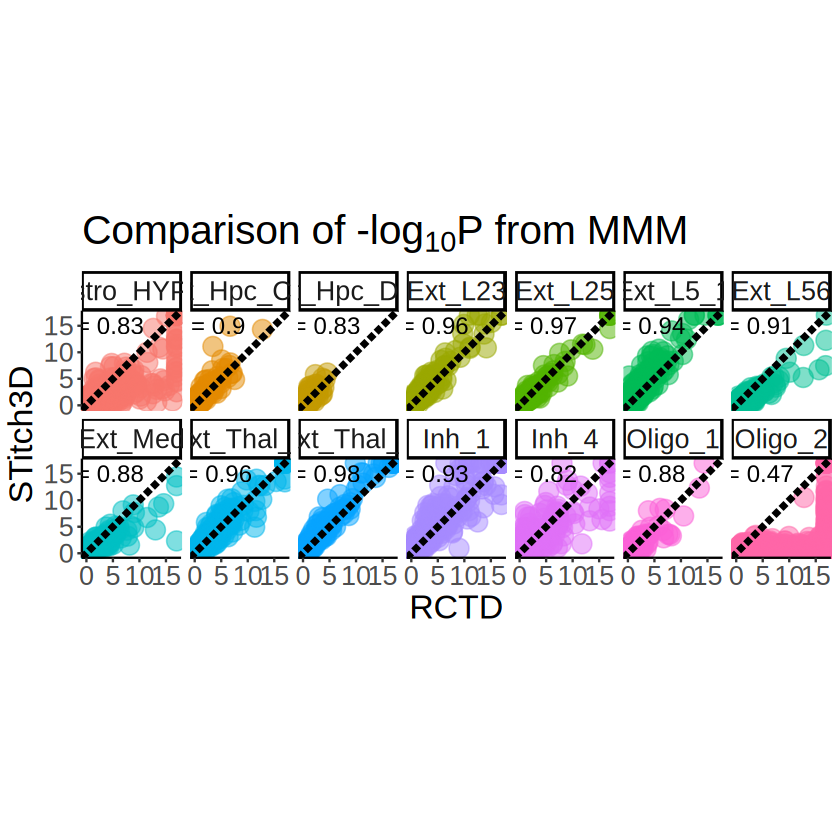
[20]:

correlations <- pvalues_merge %>%
    group_by(celltype) %>%
    summarize(
        correlation = cor(minus_log10_pvalue_RCTD, minus_log10_pvalue_ST, method = "pearson")
    )

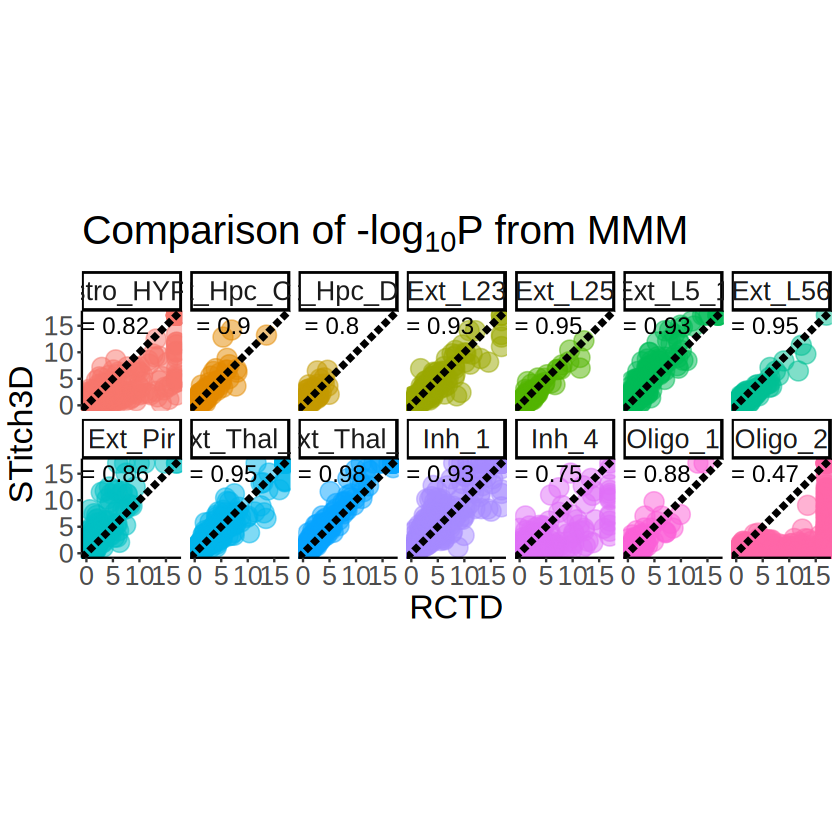
[21]:

p <- ggplot(pvalues_merge, aes(x = minus_log10_pvalue_RCTD, y = minus_log10_pvalue_ST)) +
    geom_point(aes(color = celltype), size = 5, alpha = 0.5) +
    geom_abline(slope = 1, intercept = 0, linetype = "longdash", color = "black", linewidth = 1.5) +
    geom_text(
        data = correlations,
        mapping = aes(
            x = 4, y = 15,
            label = paste("r =", round(correlation, 2))
        ),
        size = 5
    ) +
    scale_x_continuous(limits = c(0, 17), oob = scales::oob_squish) +
    scale_y_continuous(limits = c(0, 17), oob = scales::oob_squish) +
    coord_fixed(ratio = 1) +
    labs(
        title = expression(paste("Comparison of ", "-log"[10], plain("P"), " from MMM")),
        x = "RCTD", y = "STitch3D"
    ) +
    facet_wrap(celltype ~ ., nrow = 2) +
    theme_classic() +
    theme(
        plot.title = element_text(size = 24),
        axis.text.x = element_text(size = 16),
        axis.text.y = element_text(size = 16),
        axis.title.x = element_text(size = 20),
        axis.title.y = element_text(size = 20),
        strip.text = element_text(size = 16),
        legend.title = element_blank(),
        legend.text = element_text(size = 16),
        legend.position = "none"
    )
ggsave(
    file.path(RESULT_PATH, "visium_1", "MMM_RCTD_vs_STitch3D.pdf"),
    plot = p,
    width = 15, height = 6
)
ggsave(
    file.path(RESULT_PATH, "visium_1", "MMM_RCTD_vs_STitch3D.png"),
    plot = p,
    width = 15, height = 6
)
p

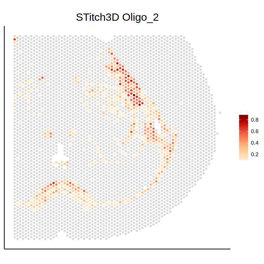
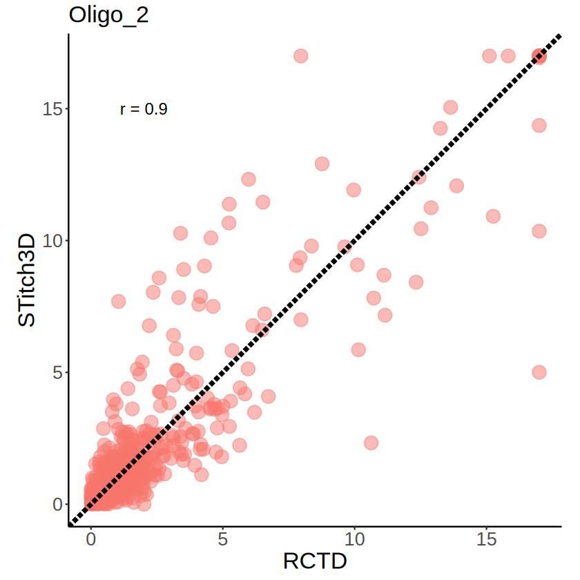
../../_images/analysis_mouse_brain_mouse_brain_MCube_reliability_31_0.png

Detailed comparison of Oligo_2

[22]:

# mcube_object_RCTD_1 <- readRDS(
#     file = file.path(
#         RESULT_PATH, "visium_1",
#         paste0("mcube_RCTD", ".rds")
#     )
# )
# mcube_object_ST_1 <- readRDS(
#     file = file.path(
#         RESULT_PATH, "visium_1",
#         paste0("mcube_ST", ".rds")
#     )
# )

[23]:

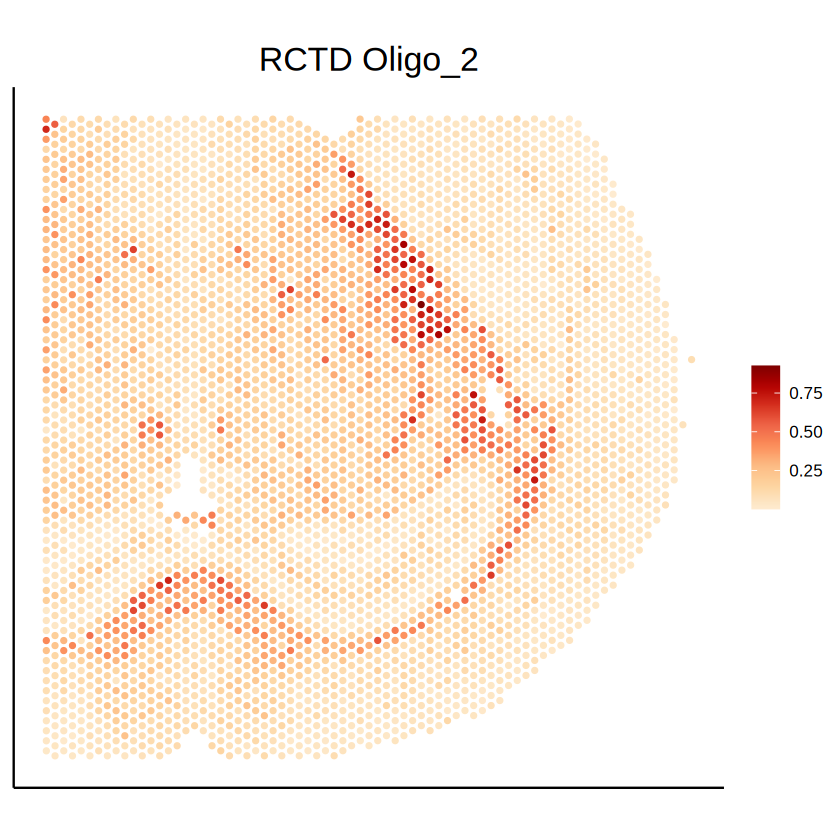
celltype <- "Oligo_2"

p1 <- mcubePlotPropCellType(mcube_object_RCTD_1@proportions, mcube_object_RCTD_1@coordinates, celltype) +
    labs(title = paste("RCTD", celltype)) +
    theme(
        text = element_text(size = 1, hjust = 0.5),
        plot.title = element_text(size = 20, hjust = 0.5),
        axis.title = element_blank(),
        axis.text.x = element_blank(),
        axis.text.y = element_blank(),
        axis.ticks = element_blank(),
        legend.text = element_text(size = 10),
        legend.position = "right"
    )
ggsave(
    filename = file.path(RESULT_PATH, paste0("proportion_", celltype, "_RCTD", ".pdf")),
    plot = p1, width = 4, height = 4
)

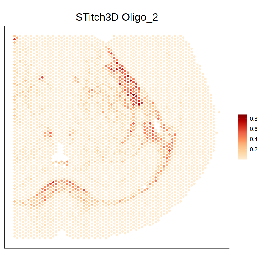
p2 <- mcubePlotPropCellType(mcube_object_ST_1@proportions, mcube_object_ST_1@coordinates, celltype) +
    labs(title = paste("STitch3D", celltype)) +
    theme(
        text = element_text(size = 1, hjust = 0.5),
        plot.title = element_text(size = 20, hjust = 0.5),
        axis.title = element_blank(),
        axis.text.x = element_blank(),
        axis.text.y = element_blank(),
        axis.ticks = element_blank(),
        legend.text = element_text(size = 10),
        legend.position = "right"
    )
ggsave(
    filename = file.path(RESULT_PATH, paste0("proportion_", celltype, "_STitch3D", ".pdf")),
    plot = p2, width = 4, height = 4
)

p1
p2

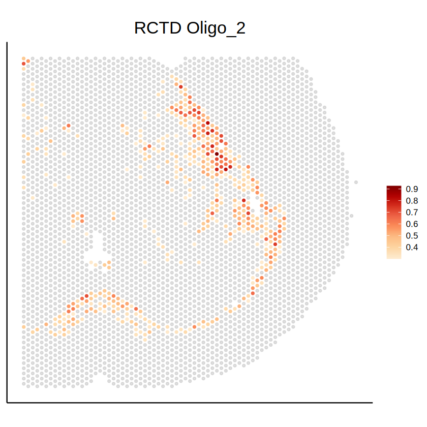
../../_images/analysis_mouse_brain_mouse_brain_MCube_reliability_34_0.png

../../_images/analysis_mouse_brain_mouse_brain_MCube_reliability_34_1.png

[24]:

p1 <- mcubePlotPropCellType(
    mcube_object_RCTD_1@proportions, mcube_object_RCTD_1@coordinates, celltype,
    background = TRUE, proportion_threshold = 0.3
) +
labs(title = paste("RCTD", celltype)) +
    theme(
        text = element_text(size = 1, hjust = 0.5),
        plot.title = element_text(size = 20, hjust = 0.5),
        axis.title = element_blank(),
        axis.text.x = element_blank(),
        axis.text.y = element_blank(),
        axis.ticks = element_blank(),
        legend.text = element_text(size = 10),
        legend.position = "right"
    )
ggsave(
    filename = file.path(
        RESULT_PATH, "visium_1",
        paste0("proportion_", celltype, "_region_RCTD", ".pdf")
    ),
    plot = p1, width = 4, height = 4
)
p2 <- mcubePlotPropCellType(
    mcube_object_ST_1@proportions, mcube_object_ST_1@coordinates,
    celltype, background = TRUE) +
    labs(title = paste("STitch3D", celltype)) +
        theme(
            text = element_text(size = 1, hjust = 0.5),
            plot.title = element_text(size = 20, hjust = 0.5),
            axis.title = element_blank(),
            axis.text.x = element_blank(),
            axis.text.y = element_blank(),
            axis.ticks = element_blank(),
            legend.text = element_text(size = 10),
            legend.position = "right"
        )
ggsave(
    filename = file.path(
        RESULT_PATH, "visium_1",
        paste0("proportion_", celltype, "_region_STitch3D", ".pdf")
    ),
    plot = p2, width = 4, height = 4
)
p1
p2

../../_images/analysis_mouse_brain_mouse_brain_MCube_reliability_35_0.png

../../_images/analysis_mouse_brain_mouse_brain_MCube_reliability_35_1.png

[25]:

mcube_region_RCTD <- createMCube(
    counts = t(as.matrix(myRCTD@originalSpatialRNA@counts[, spot_names])),
    coordinates = as.matrix(myRCTD@spatialRNA@coords),
    proportions = weights_RCTD / rowSums(weights_RCTD),
    library_sizes = myRCTD@spatialRNA@nUMI,
    reference = t(myRCTD@cell_type_info$info[[1]]),
    used_for_deconvolution = rownames(myRCTD@spatialRNA@counts),
    spot_effects = spot_effects_RCTD,
    celltype_test = "Oligo_2",
    celltype_threshold = 50, proportion_threshold = 0.3,
    project = "mouse_brain_visium_1"
)
mcube_region_RCTD <- mcubeFitNull(
    mcube_region_RCTD,
    num_workers = 36, num_threads = 1
)
mcube_region_RCTD <- mcubeTest(
    mcube_region_RCTD,
    num_workers = 36, num_threads = 1, shared_memory = TRUE
)

The batch_id is not provided!
All spots are assumed to be from the same batch and share the same gene platform effects.

Select high-abundance cell types to analyze with proportion_threshold = 0.3 and celltype_threshold = 50.

mcubeFilterCellTypes: Cell type(s) Ext_L23, Oligo_2, Inh_1, Ext_Thal_1, Ext_L56, Ext_Thal_2, Ext_Hpc_DG1, Ext_Hpc_CA1 pass the threshold.

Cell type(s) Oligo_2 will be analyzed.

Filter out lowly-expressed genes with gene_threshold = 5e-05.

mcubeFilterGenes: 2768 genes pass the threshold.

The platform effects are not provided and need to be estimated from data!

Select highly-expressed genes to analyze for each specific cell type with reference_threshold = 0.5.

mcubeFilterGenesCellType: Select 1347 genes to analyze for Oligo_2.

Preprocessed data description: 4167 spots and 58 cell types in total. 483 spots, 1347 genes, and 1 cell type(s) to analyze.

Number of physical cores: 40.

Number of workers: 36.

Number of thread(s) on BLAS per worker: 1.

mcubeKernel: length_scale is set as 0.101063440730398 for the Gaussian kernel.

mcubeKernel: length_scale is set as 0.142925288541018 for the Gaussian kernel.

mcubeKernel: length_scale is set as 0.101063440730398 for the Gaussian_transformed kernel.

mcubeKernel: length_scale is set as 0.142925288541018 for the Gaussian_transformed kernel.

Number of physical cores: 40.

Number of workers: 36.

Number of thread(s) on BLAS per worker: 1.

[26]:

mcube_region_ST <- createMCube(
    counts = counts,
    coordinates = coordinates,
    proportions = proportions_ST,
    library_sizes = library_sizes_ST,
    reference = reference_ST,
    spot_effects = spot_effects_ST,
    celltype_test = "Oligo_2",
    celltype_threshold = 50,
    project = "mouse_brain_visium_1"
)
mcube_region_ST <- mcubeFitNull(
    mcube_region_ST,
    num_workers = 36, num_threads = 1
)
mcube_region_ST <- mcubeTest(
    mcube_region_ST,
    num_workers = 36, num_threads = 1, shared_memory = TRUE
)

The batch_id is not provided!
All spots are assumed to be from the same batch and share the same gene platform effects.

Select high-abundance cell types to analyze with proportion_threshold = 0.1 and celltype_threshold = 50.

mcubeFilterCellTypes: Cell type(s) Astro_HYPO, Ext_Amy_2, Ext_Hpc_CA1, Ext_Hpc_DG1, Ext_L23, Ext_L25, Ext_L56, Ext_L5_1, Ext_L5_2, Ext_Pir, Ext_Thal_1, Ext_Thal_2, Ext_Unk_3, Inh_1, Inh_2, Inh_3, Inh_4, Oligo_1, Oligo_2 pass the threshold.

Cell type(s) Oligo_2 will be analyzed.

Filter out lowly-expressed genes with gene_threshold = 5e-05.

mcubeFilterGenes: 2599 genes pass the threshold.

The platform effects are not provided and need to be estimated from data!

Select highly-expressed genes to analyze for each specific cell type with reference_threshold = 0.5.

mcubeFilterGenesCellType: Select 991 genes to analyze for Oligo_2.

Preprocessed data description: 4168 spots and 58 cell types in total. 628 spots, 991 genes, and 1 cell type(s) to analyze.

Number of physical cores: 40.

Number of workers: 36.

Number of thread(s) on BLAS per worker: 1.

mcubeKernel: length_scale is set as 0.101059327818091 for the Gaussian kernel.

mcubeKernel: length_scale is set as 0.142919472004653 for the Gaussian kernel.

mcubeKernel: length_scale is set as 0.101059327818091 for the Gaussian_transformed kernel.

mcubeKernel: length_scale is set as 0.142919472004653 for the Gaussian_transformed kernel.

Number of physical cores: 40.

Number of workers: 36.

Number of thread(s) on BLAS per worker: 1.

[27]:

mcube_pvalues_region_RCTD <- mcubePvalueList2LongTable(mcube_region_RCTD@pvalues)
mcube_pvalues_region_RCTD$minus_log10_pvalue <- -log10(mcube_pvalues_region_RCTD$pvalue)
mcube_pvalues_region_RCTD$minus_log10_pvalue[mcube_pvalues_region_RCTD$minus_log10_pvalue > 17] <- 17
mcube_pvalues_region_ST <- mcubePvalueList2LongTable(mcube_region_ST@pvalues)
mcube_pvalues_region_ST$minus_log10_pvalue <- -log10(mcube_pvalues_region_ST$pvalue)
mcube_pvalues_region_ST$minus_log10_pvalue[mcube_pvalues_region_ST$minus_log10_pvalue > 17] <- 17
pvalues_merge <- merge(
    mcube_pvalues_region_RCTD, mcube_pvalues_region_ST,
    by = c("celltype", "gene"),
    suffixes = c("_RCTD", "_ST")
)
head(pvalues_merge)

A data.frame: 6 × 6
	celltype	gene	pvalue_RCTD	minus_log10_pvalue_RCTD	pvalue_ST	minus_log10_pvalue_ST
	<chr>	<chr>	<dbl>	<dbl>	<dbl>	<dbl>
1	Oligo_2	1110004F10Rik	0.01716477	1.76536211	1.537800e-01	0.8131003
2	Oligo_2	1110051M20Rik	0.01430794	1.84442276	3.843169e-02	1.4153105
3	Oligo_2	1700025G04Rik	0.54033421	0.26733754	4.166653e-01	0.3802126
4	Oligo_2	4930402H24Rik	0.01426273	1.84579720	1.176651e-05	4.9293522
5	Oligo_2	4931406P16Rik	0.87411995	0.05842897	5.004367e-01	0.3006508
6	Oligo_2	4933431E20Rik	0.15644749	0.80563139	4.845538e-02	1.3146580

[28]:

correlation <- cor(
    pvalues_merge$minus_log10_pvalue_RCTD, pvalues_merge$minus_log10_pvalue_ST,
    method = "pearson"
)

[29]:

p <- ggplot(pvalues_merge, aes(x = minus_log10_pvalue_RCTD, y = minus_log10_pvalue_ST)) +
  geom_point(aes(color = celltype), size = 5, alpha = 0.5) +
  geom_abline(slope = 1, intercept = 0, linetype = "longdash", color = "black", linewidth = 1.5) +
  annotate(
    "text",
    label = paste("r =", round(correlation, 2)),
    x = 2, y = 15, size = 5
  ) +
    scale_x_continuous(limits = c(0, 17), oob = scales::oob_squish) +
    scale_y_continuous(limits = c(0, 17), oob = scales::oob_squish) +
    coord_fixed(ratio = 1) +
    labs(
        title = celltype,
        x = "RCTD", y = "STitch3D"
    ) +
    theme_classic() +
    theme(
        plot.title = element_text(size = 20),
        axis.text.x = element_text(size = 16),
        axis.text.y = element_text(size = 16),
        axis.title.x = element_text(size = 20),
        axis.title.y = element_text(size = 20),
        legend.position = "none"
    )
ggsave(
  file.path(RESULT_PATH, "visium_1", "MMM_Oligo_2_RCTD_vs_STitch3D.pdf"),
  plot = p,
  width = 4, height = 4
)
p

../../_images/analysis_mouse_brain_mouse_brain_MCube_reliability_40_0.png

[30]:

rm(mcube_object_RCTD_1, mcube_object_ST_1)

Visium Slice 2

[31]:

counts <- as.data.frame(readr::read_csv(
    file.path(RAW_DATA_PATH, "visium_2", "counts.csv")
))
rownames(counts) <- counts[, 1]
counts[, 1] <- NULL
counts <- as.matrix(counts)
dim(counts)

coordinates <- as.data.frame(readr::read_csv(
    file.path(RAW_DATA_PATH, "visium_2", "3D_coordinates.csv")
))
rownames(coordinates) <- coordinates[, 1]
coordinates[, c(1, 4)] <- NULL
coordinates <- as.matrix(coordinates)
dim(coordinates)

puck <- SpatialRNA(as.data.frame(coordinates), t(counts), rowSums(counts))

New names:
• `` -> `...1`
Rows: 3925 Columns: 6416
── Column specification ────────────────────────────────────────────────────────
Delimiter: ","
chr    (1): ...1
dbl (6415): 0610040J01Rik, 0610043K17Rik, 1110002J07Rik, 1110004F10Rik, 1110...

ℹ Use `spec()` to retrieve the full column specification for this data.
ℹ Specify the column types or set `show_col_types = FALSE` to quiet this message.

3925
6415

New names:
• `` -> `...1`
Rows: 3925 Columns: 4
── Column specification ────────────────────────────────────────────────────────
Delimiter: ","
chr (1): ...1
dbl (3): x, y, z

ℹ Use `spec()` to retrieve the full column specification for this data.
ℹ Specify the column types or set `show_col_types = FALSE` to quiet this message.

3925
2

Integrating with `RCTD`

Cell type deconvolution

[32]:

# minor_celltypes <- names(which(table(sc_labels) < 25))
myRCTD <- create.RCTD(
    puck, reference,
    CELL_MIN_INSTANCE = 20, max_cores = 8
)
myRCTD <- run.RCTD(myRCTD, doublet_mode = "full")
saveRDS(myRCTD, file.path(RESULT_PATH, "visium_2", "myRCTD.rds"))
# myRCTD <- readRDS(file.path(RESULT_PATH, "visium_2", "myRCTD.rds"))

Begin: process_cell_type_info

process_cell_type_info: number of cells in reference: 38849

process_cell_type_info: number of genes in reference: 6415


       Ext_L23        Oligo_2 Astro_THAL_med        Inh_Sst          Inh_6
          1244          10000            405            640            467
      Ext_L5_3    Inh_Meis2_3          Micro       Ext_L5_2        Ext_Pir
           127            789           1218            166            954
     Astro_AMY          Inh_2          Inh_1      Inh_Pvalb      Inh_Lamp5
           498            839            573            804            331
       Ext_L25           Nb_2     Ext_Thal_1        Ext_L56      Ext_Unk_2
           922            203           1197           1422            205
     Ext_Unk_3          Inh_3      Ext_Amy_2     Ext_Thal_2       Ext_L5_1
           416            818            797            671            893
         OPC_1  Astro_AMY_CTX    Ext_Hpc_DG1     Astro_HYPO          Inh_4
          1015            279            554            451           1389
   Inh_Meis2_1    Ext_Hpc_DG2        Ext_Med    Inh_Meis2_2    Ext_Hpc_CA1
           363            915             70            602            671
       Ext_L6B      Astro_CTX      Ext_Amy_1       Astro_WM        Oligo_1
           356            443            519            220            613
     Astro_STR         Ext_L6 Astro_THAL_lat           Nb_1         LowQ_2
            81            568            332            225            265
       Inh_Vip      Astro_HPC    Ext_ClauPyr    Ext_Hpc_CA2          OPC_2
           545            261            272             48            300
         Inh_5    Ext_Hpc_CA3      Ext_Unk_1    Inh_Meis2_4          Unk_2
           118            232             90            193             85
Astro_THAL_hab         LowQ_1           Endo
            43            110             22

End: process_cell_type_info

create.RCTD: getting regression differentially expressed genes:

get_de_genes: Ext_L23 found DE genes: 112

get_de_genes: Oligo_2 found DE genes: 408

get_de_genes: Astro_THAL_med found DE genes: 353

get_de_genes: Inh_Sst found DE genes: 123

get_de_genes: Inh_6 found DE genes: 195

get_de_genes: Ext_L5_3 found DE genes: 133

get_de_genes: Inh_Meis2_3 found DE genes: 153

get_de_genes: Micro found DE genes: 647

get_de_genes: Ext_L5_2 found DE genes: 102

get_de_genes: Ext_Pir found DE genes: 69

get_de_genes: Astro_AMY found DE genes: 333

get_de_genes: Inh_2 found DE genes: 99

get_de_genes: Inh_1 found DE genes: 86

get_de_genes: Inh_Pvalb found DE genes: 132

get_de_genes: Inh_Lamp5 found DE genes: 167

get_de_genes: Ext_L25 found DE genes: 147

get_de_genes: Nb_2 found DE genes: 364

get_de_genes: Ext_Thal_1 found DE genes: 212

get_de_genes: Ext_L56 found DE genes: 157

get_de_genes: Ext_Unk_2 found DE genes: 150

get_de_genes: Ext_Unk_3 found DE genes: 150

get_de_genes: Inh_3 found DE genes: 88

get_de_genes: Ext_Amy_2 found DE genes: 74

get_de_genes: Ext_Thal_2 found DE genes: 151

get_de_genes: Ext_L5_1 found DE genes: 105

get_de_genes: OPC_1 found DE genes: 247

get_de_genes: Astro_AMY_CTX found DE genes: 348

get_de_genes: Ext_Hpc_DG1 found DE genes: 196

get_de_genes: Astro_HYPO found DE genes: 352

get_de_genes: Inh_4 found DE genes: 83

get_de_genes: Inh_Meis2_1 found DE genes: 127

get_de_genes: Ext_Hpc_DG2 found DE genes: 184

get_de_genes: Ext_Med found DE genes: 109

get_de_genes: Inh_Meis2_2 found DE genes: 156

get_de_genes: Ext_Hpc_CA1 found DE genes: 185

get_de_genes: Ext_L6B found DE genes: 155

get_de_genes: Astro_CTX found DE genes: 330

get_de_genes: Ext_Amy_1 found DE genes: 112

get_de_genes: Astro_WM found DE genes: 315

get_de_genes: Oligo_1 found DE genes: 355

get_de_genes: Astro_STR found DE genes: 343

get_de_genes: Ext_L6 found DE genes: 95

get_de_genes: Astro_THAL_lat found DE genes: 328

get_de_genes: Nb_1 found DE genes: 239

get_de_genes: LowQ_2 found DE genes: 157

get_de_genes: Inh_Vip found DE genes: 120

get_de_genes: Astro_HPC found DE genes: 337

get_de_genes: Ext_ClauPyr found DE genes: 135

get_de_genes: Ext_Hpc_CA2 found DE genes: 154

get_de_genes: OPC_2 found DE genes: 358

get_de_genes: Inh_5 found DE genes: 172

get_de_genes: Ext_Hpc_CA3 found DE genes: 135

get_de_genes: Ext_Unk_1 found DE genes: 181

get_de_genes: Inh_Meis2_4 found DE genes: 166

get_de_genes: Unk_2 found DE genes: 172

get_de_genes: Astro_THAL_hab found DE genes: 378

get_de_genes: LowQ_1 found DE genes: 416

get_de_genes: Endo found DE genes: 648

get_de_genes: total DE genes: 3432

create.RCTD: getting platform effect normalization differentially expressed genes:

get_de_genes: Ext_L23 found DE genes: 281

get_de_genes: Oligo_2 found DE genes: 585

get_de_genes: Astro_THAL_med found DE genes: 595

get_de_genes: Inh_Sst found DE genes: 234

get_de_genes: Inh_6 found DE genes: 391

get_de_genes: Ext_L5_3 found DE genes: 315

get_de_genes: Inh_Meis2_3 found DE genes: 332

get_de_genes: Micro found DE genes: 969

get_de_genes: Ext_L5_2 found DE genes: 267

get_de_genes: Ext_Pir found DE genes: 214

get_de_genes: Astro_AMY found DE genes: 578

get_de_genes: Inh_2 found DE genes: 276

get_de_genes: Inh_1 found DE genes: 289

get_de_genes: Inh_Pvalb found DE genes: 302

get_de_genes: Inh_Lamp5 found DE genes: 337

get_de_genes: Ext_L25 found DE genes: 327

get_de_genes: Nb_2 found DE genes: 719

get_de_genes: Ext_Thal_1 found DE genes: 402

get_de_genes: Ext_L56 found DE genes: 334

get_de_genes: Ext_Unk_2 found DE genes: 317

get_de_genes: Ext_Unk_3 found DE genes: 315

get_de_genes: Inh_3 found DE genes: 267

get_de_genes: Ext_Amy_2 found DE genes: 225

get_de_genes: Ext_Thal_2 found DE genes: 326

get_de_genes: Ext_L5_1 found DE genes: 275

get_de_genes: OPC_1 found DE genes: 431

get_de_genes: Astro_AMY_CTX found DE genes: 599

get_de_genes: Ext_Hpc_DG1 found DE genes: 376

get_de_genes: Astro_HYPO found DE genes: 591

get_de_genes: Inh_4 found DE genes: 303

get_de_genes: Inh_Meis2_1 found DE genes: 323

get_de_genes: Ext_Hpc_DG2 found DE genes: 361

get_de_genes: Ext_Med found DE genes: 298

get_de_genes: Inh_Meis2_2 found DE genes: 348

get_de_genes: Ext_Hpc_CA1 found DE genes: 323

get_de_genes: Ext_L6B found DE genes: 332

get_de_genes: Astro_CTX found DE genes: 545

get_de_genes: Ext_Amy_1 found DE genes: 295

get_de_genes: Astro_WM found DE genes: 566

get_de_genes: Oligo_1 found DE genes: 521

get_de_genes: Astro_STR found DE genes: 577

get_de_genes: Ext_L6 found DE genes: 286

get_de_genes: Astro_THAL_lat found DE genes: 570

get_de_genes: Nb_1 found DE genes: 523

get_de_genes: LowQ_2 found DE genes: 308

get_de_genes: Inh_Vip found DE genes: 252

get_de_genes: Astro_HPC found DE genes: 572

get_de_genes: Ext_ClauPyr found DE genes: 299

get_de_genes: Ext_Hpc_CA2 found DE genes: 292

get_de_genes: OPC_2 found DE genes: 551

get_de_genes: Inh_5 found DE genes: 389

get_de_genes: Ext_Hpc_CA3 found DE genes: 255

get_de_genes: Ext_Unk_1 found DE genes: 397

get_de_genes: Inh_Meis2_4 found DE genes: 345

get_de_genes: Unk_2 found DE genes: 377

get_de_genes: Astro_THAL_hab found DE genes: 689

get_de_genes: LowQ_1 found DE genes: 811

get_de_genes: Endo found DE genes: 999

get_de_genes: total DE genes: 4489

fitBulk: decomposing bulk

chooseSigma: using initial Q_mat with sigma =  1

Likelihood value: 3477085.10018692

Sigma value:  0.84

Likelihood value: 3407256.54450731

Sigma value:  0.69

Likelihood value: 3350849.20022504

Sigma value:  0.61

Likelihood value: 3326070.00234539

Sigma value:  0.53

Likelihood value: 3306210.96510287

Sigma value:  0.45

Likelihood value: 3292424.52368184

Sigma value:  0.37

Likelihood value: 3286007.90768412

Sigma value:  0.35

Likelihood value: 3285716.09270385

Sigma value:  0.35

[33]:

write.table(
    rownames(myRCTD@spatialRNA@counts),
    file = file.path(
        DATA_PATH, "visium_2",
        paste0("HVG_RCTD", ".csv")
    ),
    quote = FALSE, row.names = FALSE, col.names = FALSE
)

[34]:

weights_RCTD <- as.matrix(myRCTD@results$weights)
proportions_RCTD <- weights_RCTD / rowSums(weights_RCTD)

proportions_filter <- proportions_RCTD
proportions_filter[proportions_filter < 0.1] <- 0
major_celltypes <- colnames(proportions_filter)[
    which(colSums(proportions_filter) > 50)
]

proportions_RCTD_long_2 <- proportions_RCTD[, major_celltypes] %>%
  cbind(myRCTD@spatialRNA@coords) %>%
  tidyr::pivot_longer(
    cols = -(x:y),
    names_to = "Cell type",
    values_to = "Proportion"
  )
head(proportions_RCTD_long_2)

A tibble: 6 × 4
x	y	Cell type	Proportion
<dbl>	<dbl>	<chr>	<dbl>
4359.614	5109.826	Ext_L23	1.971831e-05
4359.614	5109.826	Oligo_2	7.585819e-02
4359.614	5109.826	Inh_1	1.971831e-05
4359.614	5109.826	Ext_L25	5.911649e-02
4359.614	5109.826	Ext_Thal_1	1.971831e-05
4359.614	5109.826	Ext_L56	1.298476e-01

[35]:

p <- ggplot(proportions_RCTD_long_2, aes(x = x, y = y)) +
    geom_point(aes(color = Proportion), size = 1, alpha = 1) +
    scale_colour_gradientn(name = NULL, colors = pals::brewer.orrd(22)[3:22]) +
    scale_y_continuous(trans = "reverse") +
    coord_fixed(ratio = 1) +
    facet_wrap(~`Cell type`, ncol = 6) +
    labs(
        title = "Estimated cell type proportions by RCTD",
        x = "x", y = "y"
    ) +
    theme_classic() +
    theme(
        plot.title = element_text(size = 24, hjust = 0.5),
        axis.text.x = element_text(size = 16),
        axis.text.y = element_text(size = 16),
        axis.title.x = element_blank(),
        axis.title.y = element_blank(),
        strip.text = element_text(size = 16),
        legend.title = element_blank(),
        legend.text = element_text(size = 16),
        legend.position = "right"
    )
ggsave(
    filename = file.path(RESULT_PATH, "visium_2", "proportions_RCTD.pdf"),
    plot = p, width = 16, height = 9
)

Identifying cell-type-specific SVGs using `MCube`

[36]:

spot_names <- colnames(myRCTD@spatialRNA@counts)
weights_RCTD <- as.matrix(myRCTD@results$weights)
spot_effects_RCTD <- log(rowSums(weights_RCTD))
names(spot_effects_RCTD) <- rownames(weights_RCTD)

[37]:

mcube_object_RCTD_2 <- createMCube(
    counts = t(as.matrix(myRCTD@originalSpatialRNA@counts[, spot_names])),
    coordinates = as.matrix(myRCTD@spatialRNA@coords),
    proportions = weights_RCTD / rowSums(weights_RCTD),
    library_sizes = myRCTD@spatialRNA@nUMI,
    reference = t(myRCTD@cell_type_info$info[[1]]),
    used_for_deconvolution = rownames(myRCTD@spatialRNA@counts),
    spot_effects = spot_effects_RCTD,
    celltype_test = grep("Unk|LowQ", levels(sc_labels), value = TRUE, invert = TRUE),
    celltype_threshold = 50,
    project = "mouse_brain_visium_2"
)
mcube_object_RCTD_2 <- mcubeFitNull(
    mcube_object_RCTD_2,
    num_workers = 36, num_threads = 1
)
mcube_object_RCTD_2 <- mcubeTest(
    mcube_object_RCTD_2,
    num_workers = 36, num_threads = 1, shared_memory = TRUE
)

saveRDS(
    mcube_object_RCTD_2,
    file = file.path(
        RESULT_PATH, "visium_2",
        paste0("mcube_RCTD", ".rds")
    )
)
saveRDS(
    mcube_object_RCTD_2@pvalues,
    file = file.path(
        RESULT_PATH, "visium_2",
        paste0("mcube_pvalues_RCTD", ".rds")
    )
)
rm(mcube_object_RCTD_2)

# mcube_pvalues_RCTD_2 <- readRDS(
#     file = file.path(
#         RESULT_PATH, "visium_2",
#         paste0("mcube_pvalues_RCTD", ".rds")
#     )
# )

The batch_id is not provided!
All spots are assumed to be from the same batch and share the same gene platform effects.

Select high-abundance cell types to analyze with proportion_threshold = 0.1 and celltype_threshold = 50.

mcubeFilterCellTypes: Cell type(s) Ext_L23, Oligo_2, Inh_1, Ext_L25, Ext_Thal_1, Ext_L56, Ext_Thal_2, Ext_L5_1, Ext_Hpc_DG1, Astro_HYPO, Inh_4, Ext_Med, Ext_Hpc_CA1, Oligo_1, Astro_HPC pass the threshold.

Cell type(s) Astro_THAL_med, Inh_Sst, Inh_6, Ext_L5_3, Inh_Meis2_3, Micro, Ext_L5_2, Ext_Pir, Astro_AMY, Inh_2, Inh_Pvalb, Inh_Lamp5, Nb_2, Inh_3, Ext_Amy_2, OPC_1, Astro_AMY_CTX, Inh_Meis2_1, Ext_Hpc_DG2, Inh_Meis2_2, Ext_L6B, Astro_CTX, Ext_Amy_1, Astro_WM, Astro_STR, Ext_L6, Astro_THAL_lat, Nb_1, Inh_Vip, Ext_ClauPyr, Ext_Hpc_CA2, OPC_2, Inh_5, Ext_Hpc_CA3, Inh_Meis2_4, Astro_THAL_hab, Endo has/have less than the minimum celltype_threshold = 50 with proportion_threshold = 0.1.
To include the above cell type(s), please reduce celltype_threshold or proportion_threshold.

Cell type(s) Ext_L23, Oligo_2, Inh_1, Ext_L25, Ext_Thal_1, Ext_L56, Ext_Thal_2, Ext_L5_1, Ext_Hpc_DG1, Astro_HYPO, Inh_4, Ext_Med, Ext_Hpc_CA1, Oligo_1, Astro_HPC will be analyzed.

Filter out lowly-expressed genes with gene_threshold = 5e-05.

mcubeFilterGenes: 2767 genes pass the threshold.

The platform effects are not provided and need to be estimated from data!

Select highly-expressed genes to analyze for each specific cell type with reference_threshold = 0.5.

mcubeFilterGenesCellType: Select 954 genes to analyze for Ext_L23.

mcubeFilterGenesCellType: Select 1073 genes to analyze for Oligo_2.

mcubeFilterGenesCellType: Select 1161 genes to analyze for Inh_1.

mcubeFilterGenesCellType: Select 989 genes to analyze for Ext_L25.

mcubeFilterGenesCellType: Select 938 genes to analyze for Ext_Thal_1.

mcubeFilterGenesCellType: Select 1024 genes to analyze for Ext_L56.

mcubeFilterGenesCellType: Select 1041 genes to analyze for Ext_Thal_2.

mcubeFilterGenesCellType: Select 967 genes to analyze for Ext_L5_1.

mcubeFilterGenesCellType: Select 981 genes to analyze for Ext_Hpc_DG1.

mcubeFilterGenesCellType: Select 1137 genes to analyze for Astro_HYPO.

mcubeFilterGenesCellType: Select 1162 genes to analyze for Inh_4.

mcubeFilterGenesCellType: Select 1033 genes to analyze for Ext_Med.

mcubeFilterGenesCellType: Select 887 genes to analyze for Ext_Hpc_CA1.

mcubeFilterGenesCellType: Select 869 genes to analyze for Oligo_1.

mcubeFilterGenesCellType: Select 1112 genes to analyze for Astro_HPC.

Preprocessed data description: 3924 spots and 58 cell types in total. 3658 spots, 2756 genes, and 15 cell type(s) to analyze.

Number of physical cores: 40.

Number of workers: 36.

Number of thread(s) on BLAS per worker: 1.

mcubeKernel: length_scale is set as 0.104574506874699 for the Gaussian kernel.

mcubeKernel: length_scale is set as 0.147890685900678 for the Gaussian kernel.

mcubeKernel: length_scale is set as 0.104574506874699 for the Gaussian_transformed kernel.

mcubeKernel: length_scale is set as 0.147890685900678 for the Gaussian_transformed kernel.

Number of physical cores: 40.

Number of workers: 36.

Number of thread(s) on BLAS per worker: 1.

Integrating with `STitch3D`

Load in deconvolution results

[38]:

reference_ST <- data.matrix(read.csv(
    file.path(DATA_PATH, "visium_2", "reference_ST.csv"),
    header = TRUE, row.names = 1, check.names = FALSE
))
dim(reference_ST)
num_celltypes <- nrow(reference_ST)

proportions_ST <- data.matrix(read.csv(
    file.path(DATA_PATH, "visium_2", paste0("prop_slice", 0, ".csv")),
    header = TRUE, row.names = 1, check.names = FALSE
))
dim(proportions_ST)

counts <- as.data.frame(readr::read_csv(
    file.path(DATA_PATH, "visium_2", "counts.csv")
))
rownames(counts) <- counts[, 1]
counts[, 1] <- NULL
counts <- data.matrix(counts)
dim(counts)

coordinates <- data.matrix(read.csv(
    file.path(DATA_PATH, "visium_2", "3D_coordinates.csv"),
    header = TRUE, row.names = 1, check.names = FALSE
))[, c("x", "y")]
dim(coordinates)

spot_effects_ST <- data.matrix(read.csv(
    file.path(DATA_PATH, "visium_2", "spot_effects_ST.csv"),
    header = TRUE, row.names = 1, check.names = FALSE
))[, 1]

library_sizes_ST <- data.matrix(read.csv(
    file.path(DATA_PATH, "visium_2", "library_sizes_ST.csv"),
    header = TRUE, row.names = 1, check.names = FALSE
))[, 1]

58
4489

3925
58

New names:
• `` -> `...1`
Rows: 3925 Columns: 4490
── Column specification ────────────────────────────────────────────────────────
Delimiter: ","
chr    (1): ...1
dbl (4489): Xkr4, Sox17, Rgs20, Oprk1, Rb1cc1, St18, Sntg1, Adhfe1, Sgk3, Mc...

ℹ Use `spec()` to retrieve the full column specification for this data.
ℹ Specify the column types or set `show_col_types = FALSE` to quiet this message.

3925
4489

3925
2

[39]:

proportions_filter <- proportions_ST
proportions_filter[proportions_filter < 0.1] <- 0
major_celltypes <- colnames(proportions_filter)[
    which(colSums(proportions_filter) > 50)
]

proportions_ST_long_2 <- as.data.frame(proportions_ST[, major_celltypes]) %>%
  cbind(coordinates) %>%
  tidyr::pivot_longer(
    cols = -(x:y),
    names_to = "Cell type",
    values_to = "Proportion"
  )
head(proportions_ST_long_2)

A tibble: 6 × 4
x	y	Cell type	Proportion
<dbl>	<dbl>	<chr>	<dbl>
4359.614	5109.826	Astro_HYPO	1.179485e-06
4359.614	5109.826	Ext_Amy_2	7.797921e-05
4359.614	5109.826	Ext_Hpc_CA1	1.753935e-04
4359.614	5109.826	Ext_Hpc_DG1	1.280550e-07
4359.614	5109.826	Ext_L23	1.618132e-04
4359.614	5109.826	Ext_L25	6.004004e-02

[40]:

p <- ggplot(proportions_ST_long_2, aes(x = x, y = y)) +
    geom_point(aes(color = Proportion), size = 1, alpha = 1) +
    scale_colour_gradientn(name = NULL, colors = pals::brewer.orrd(22)[3:22]) +
    scale_y_continuous(trans = "reverse") +
    coord_fixed(ratio = 1) +
    facet_wrap(~`Cell type`, nrow = 3) +
    labs(
        title = "Estimated cell type proportions by STitch3D",
        x = "x", y = "y"
    ) +
    theme_classic() +
    theme(
        plot.title = element_text(size = 24, hjust = 0.5),
        axis.text.x = element_text(size = 16),
        axis.text.y = element_text(size = 16),
        axis.title.x = element_blank(),
        axis.title.y = element_blank(),
        strip.text = element_text(size = 16),
        legend.title = element_blank(),
        legend.text = element_text(size = 16),
        legend.position = "right"
    )
ggsave(
    filename = file.path(RESULT_PATH, "visium_2", "proportions_STitch3D.pdf"),
    plot = p, width = 16, height = 9
)

Identifying cell-type-specific SVGs using `MCube`

[41]:

mcube_object_ST_2 <- createMCube(
    counts = counts,
    coordinates = coordinates,
    proportions = proportions_ST,
    library_sizes = library_sizes_ST,
    reference = reference_ST,
    spot_effects = spot_effects_ST,
    celltype_test = grep("Unk|LowQ", levels(sc_labels), value = TRUE, invert = TRUE),
    celltype_threshold = 50,
    project = "mouse_brain_visium_2"
)
mcube_object_ST_2 <- mcubeFitNull(
    mcube_object_ST_2,
    num_workers = 36, num_threads = 1
)
mcube_object_ST_2 <- mcubeTest(
    mcube_object_ST_2,
    num_workers = 36, num_threads = 1, shared_memory = TRUE
)

saveRDS(
    mcube_object_ST_2,
    file = file.path(
        RESULT_PATH, "visium_2",
        paste0("mcube_ST", ".rds")
    )
)
saveRDS(
    mcube_object_ST_2@pvalues,
    file = file.path(
        RESULT_PATH, "visium_2",
        paste0("mcube_pvalues_ST", ".rds")
    )
)
rm(mcube_object_ST_2)

# mcube_pvalues_ST_2 <- readRDS(
#     file = file.path(
#         RESULT_PATH, "sensitivity", "visium_2",
#         paste0("mcube_pvalues_ST", ".rds")
#     )
# )

The batch_id is not provided!
All spots are assumed to be from the same batch and share the same gene platform effects.

Select high-abundance cell types to analyze with proportion_threshold = 0.1 and celltype_threshold = 50.

mcubeFilterCellTypes: Cell type(s) Astro_HYPO, Ext_Amy_2, Ext_Hpc_CA1, Ext_Hpc_DG1, Ext_L23, Ext_L25, Ext_L56, Ext_L5_1, Ext_L5_2, Ext_Med, Ext_Thal_1, Ext_Thal_2, Ext_Unk_3, Inh_1, Inh_2, Inh_3, Inh_4, Oligo_1, Oligo_2 pass the threshold.

Cell type(s) Astro_AMY, Astro_AMY_CTX, Astro_CTX, Astro_HPC, Astro_STR, Astro_THAL_hab, Astro_THAL_lat, Astro_THAL_med, Astro_WM, Endo, Ext_Amy_1, Ext_ClauPyr, Ext_Hpc_CA2, Ext_Hpc_CA3, Ext_Hpc_DG2, Ext_L5_3, Ext_L6, Ext_L6B, Ext_Pir, Inh_5, Inh_6, Inh_Lamp5, Inh_Meis2_1, Inh_Meis2_2, Inh_Meis2_3, Inh_Meis2_4, Inh_Pvalb, Inh_Sst, Inh_Vip, Micro, Nb_1, Nb_2, OPC_1, OPC_2 has/have less than the minimum celltype_threshold = 50 with proportion_threshold = 0.1.
To include the above cell type(s), please reduce celltype_threshold or proportion_threshold.

Cell type(s) Astro_HYPO, Ext_Amy_2, Ext_Hpc_CA1, Ext_Hpc_DG1, Ext_L23, Ext_L25, Ext_L56, Ext_L5_1, Ext_L5_2, Ext_Med, Ext_Thal_1, Ext_Thal_2, Inh_1, Inh_2, Inh_3, Inh_4, Oligo_1, Oligo_2 will be analyzed.

Filter out lowly-expressed genes with gene_threshold = 5e-05.

mcubeFilterGenes: 2602 genes pass the threshold.

The platform effects are not provided and need to be estimated from data!

Select highly-expressed genes to analyze for each specific cell type with reference_threshold = 0.5.

mcubeFilterGenesCellType: Select 1074 genes to analyze for Astro_HYPO.

mcubeFilterGenesCellType: Select 917 genes to analyze for Ext_Amy_2.

mcubeFilterGenesCellType: Select 802 genes to analyze for Ext_Hpc_CA1.

mcubeFilterGenesCellType: Select 906 genes to analyze for Ext_Hpc_DG1.

mcubeFilterGenesCellType: Select 870 genes to analyze for Ext_L23.

mcubeFilterGenesCellType: Select 890 genes to analyze for Ext_L25.

mcubeFilterGenesCellType: Select 944 genes to analyze for Ext_L56.

mcubeFilterGenesCellType: Select 884 genes to analyze for Ext_L5_1.

mcubeFilterGenesCellType: Select 848 genes to analyze for Ext_L5_2.

mcubeFilterGenesCellType: Select 938 genes to analyze for Ext_Med.

mcubeFilterGenesCellType: Select 876 genes to analyze for Ext_Thal_1.

mcubeFilterGenesCellType: Select 961 genes to analyze for Ext_Thal_2.

mcubeFilterGenesCellType: Select 1079 genes to analyze for Inh_1.

mcubeFilterGenesCellType: Select 1001 genes to analyze for Inh_2.

mcubeFilterGenesCellType: Select 1069 genes to analyze for Inh_3.

mcubeFilterGenesCellType: Select 1077 genes to analyze for Inh_4.

mcubeFilterGenesCellType: Select 799 genes to analyze for Oligo_1.

mcubeFilterGenesCellType: Select 985 genes to analyze for Oligo_2.

Preprocessed data description: 3925 spots and 58 cell types in total. 3658 spots, 2586 genes, and 18 cell type(s) to analyze.

Number of physical cores: 40.

Number of workers: 36.

Number of thread(s) on BLAS per worker: 1.

mcubeKernel: length_scale is set as 0.104577495815249 for the Gaussian kernel.

mcubeKernel: length_scale is set as 0.147894912900941 for the Gaussian kernel.

mcubeKernel: length_scale is set as 0.104577495815249 for the Gaussian_transformed kernel.

mcubeKernel: length_scale is set as 0.147894912900941 for the Gaussian_transformed kernel.

Number of physical cores: 40.

Number of workers: 36.

Number of thread(s) on BLAS per worker: 1.

Comparison of the deconvolution results

[42]:

overlap_celltypes <- intersect(
    unique(proportions_RCTD_long_2$`Cell type`),
    unique(proportions_ST_long_2$`Cell type`)
)
overlap_celltypes <- sort(overlap_celltypes)
overlap_celltypes

'Astro_HYPO'
'Ext_Hpc_CA1'
'Ext_Hpc_DG1'
'Ext_L23'
'Ext_L25'
'Ext_L5_1'
'Ext_L56'
'Ext_Med'
'Ext_Thal_1'
'Ext_Thal_2'
'Inh_1'
'Inh_4'
'Oligo_1'
'Oligo_2'

[43]:

p <- ggplot(
    proportions_RCTD_long_2[proportions_RCTD_long_2$`Cell type` %in% overlap_celltypes, ],
    aes(x = x, y = y)
) +
    geom_point(aes(color = Proportion), size = 1, alpha = 1) +
    scale_colour_gradientn(name = NULL, colors = pals::brewer.orrd(22)[3:22]) +
    scale_y_continuous(trans = "reverse") +
    coord_fixed(ratio = 1) +
    facet_wrap(~`Cell type`, nrow = 2) +
    labs(
        title = "Estimated cell type proportions by RCTD",
        x = "x", y = "y"
    ) +
    theme_classic() +
    theme(
        plot.title = element_text(size = 24, hjust = 0.5),
        axis.text.x = element_text(size = 16),
        axis.text.y = element_text(size = 16),
        axis.title.x = element_blank(),
        axis.title.y = element_blank(),
        strip.text = element_text(size = 16),
        legend.title = element_blank(),
        legend.text = element_text(size = 16),
        legend.position = "right"
    )
ggsave(
    filename = file.path(RESULT_PATH, "visium_2", "sensitivity_proportions_RCTD.pdf"),
    plot = p, width = 16, height = 6
)

[44]:

p <- ggplot(
    proportions_ST_long_2[proportions_ST_long_2$`Cell type` %in% overlap_celltypes, ],
    aes(x = x, y = y)
) +
    geom_point(aes(color = Proportion), size = 1, alpha = 1) +
    scale_colour_gradientn(name = NULL, colors = pals::brewer.orrd(22)[3:22]) +
    scale_y_continuous(trans = "reverse") +
    coord_fixed(ratio = 1) +
    facet_wrap(~`Cell type`, nrow = 2) +
    labs(
        title = "Estimated cell type proportions by STitch3D",
        x = "x", y = "y"
    ) +
    theme_classic() +
    theme(
        plot.title = element_text(size = 24, hjust = 0.5),
        axis.text.x = element_text(size = 16),
        axis.text.y = element_text(size = 16),
        axis.title.x = element_blank(),
        axis.title.y = element_blank(),
        strip.text = element_text(size = 16),
        legend.title = element_blank(),
        legend.text = element_text(size = 16),
        legend.position = "right"
    )
ggsave(
    filename = file.path(RESULT_PATH, "visium_2", "sensitivity_proportions_STitch3D.pdf"),
    plot = p, width = 16, height = 6
)

Comparison of the cell-type-specific SVG results

[45]:

mcube_pvalues_RCTD_2 <- readRDS(
    file = file.path(
        RESULT_PATH, "visium_2",
        paste0("mcube_pvalues_RCTD", ".rds")
    )
)
mcube_pvalues_ST_2 <- readRDS(
    file = file.path(
        RESULT_PATH, "visium_2",
        paste0("mcube_pvalues_ST", ".rds")
    )
)

[46]:

mcube_pvalues_RCTD_2 <- mcubePvalueList2LongTable(mcube_pvalues_RCTD_2)
mcube_pvalues_RCTD_2$minus_log10_pvalue <- -log10(mcube_pvalues_RCTD_2$pvalue)
mcube_pvalues_RCTD_2$minus_log10_pvalue[mcube_pvalues_RCTD_2$minus_log10_pvalue > 17] <- 17
mcube_pvalues_ST_2 <- mcubePvalueList2LongTable(mcube_pvalues_ST_2)
mcube_pvalues_ST_2$minus_log10_pvalue <- -log10(mcube_pvalues_ST_2$pvalue)
mcube_pvalues_ST_2$minus_log10_pvalue[mcube_pvalues_ST_2$minus_log10_pvalue > 17] <- 17
pvalues_merge <- merge(
    mcube_pvalues_RCTD_2, mcube_pvalues_ST_2,
    by = c("celltype", "gene"),
    suffixes = c("_RCTD", "_ST")
)
head(pvalues_merge)

A data.frame: 6 × 6
	celltype	gene	pvalue_RCTD	minus_log10_pvalue_RCTD	pvalue_ST	minus_log10_pvalue_ST
	<chr>	<chr>	<dbl>	<dbl>	<dbl>	<dbl>
1	Astro_HYPO	1110004F10Rik	0.001278629	2.89325554	0.03689844	1.4329920
2	Astro_HYPO	1110051M20Rik	0.010943041	1.96086199	0.07129424	1.1469455
3	Astro_HYPO	2310022B05Rik	0.902371928	0.04461442	0.33203934	0.4788105
4	Astro_HYPO	2700081O15Rik	0.157050125	0.80396171	0.31020245	0.5083548
5	Astro_HYPO	4930402H24Rik	0.716225347	0.14495031	0.38755751	0.4116638
6	Astro_HYPO	4933431E20Rik	0.617446854	0.20940042	0.37551396	0.4253739

[47]:

correlations <- pvalues_merge %>%
    group_by(celltype) %>%
    summarize(
        correlation = cor(minus_log10_pvalue_RCTD, minus_log10_pvalue_ST, method = "pearson")
    )

[48]:

p <- ggplot(pvalues_merge, aes(x = -log10(pvalue_RCTD), y = -log10(pvalue_ST))) +
    geom_point(aes(color = celltype), size = 5, alpha = 0.5) +
    geom_abline(slope = 1, intercept = 0, linetype = "longdash", color = "black", linewidth = 1.5) +
    geom_text(
        data = correlations,
        mapping = aes(
            x = 3, y = 15,
            label = paste("r =", round(correlation, 2))
        ),
        size = 5
    ) +
    scale_x_continuous(limits = c(0, 17), oob = scales::oob_squish) +
    scale_y_continuous(limits = c(0, 17), oob = scales::oob_squish) +
    coord_fixed(ratio = 1) +
    labs(
        title = expression(paste("Comparison of ", "-log"[10], plain("P"), " from MMM")),
        x = "RCTD", y = "STitch3D"
    ) +
    facet_wrap(celltype ~ ., nrow = 2) +
    theme_classic() +
    theme(
        plot.title = element_text(size = 24),
        axis.text.x = element_text(size = 16),
        axis.text.y = element_text(size = 16),
        axis.title.x = element_text(size = 20),
        axis.title.y = element_text(size = 20),
        strip.text = element_text(size = 16),
        legend.title = element_blank(),
        legend.text = element_text(size = 16),
        legend.position = "none"
    )
ggsave(
    file.path(RESULT_PATH, "visium_2", "MMM_RCTD_vs_STitch3D.pdf"),
    plot = p,
    width = 15, height = 6
)
ggsave(
    file.path(RESULT_PATH, "visium_2", "MMM_RCTD_vs_STitch3D.png"),
    plot = p,
    width = 15, height = 6
)
p

../../_images/analysis_mouse_brain_mouse_brain_MCube_reliability_68_0.png

Replicability analysis of `MCube` using the two slices

Comparison of the deconvolution results from `RCTD` on the two slices

[49]:

overlap_celltypes <- intersect(
    unique(proportions_RCTD_long_1$`Cell type`),
    unique(proportions_RCTD_long_2$`Cell type`)
)
overlap_celltypes <- sort(overlap_celltypes)
overlap_celltypes

'Astro_HPC'
'Astro_HYPO'
'Ext_Hpc_CA1'
'Ext_Hpc_DG1'
'Ext_L23'
'Ext_L25'
'Ext_L5_1'
'Ext_L56'
'Ext_Med'
'Ext_Thal_1'
'Ext_Thal_2'
'Inh_1'
'Inh_4'
'Oligo_1'
'Oligo_2'

[50]:

p <- ggplot(
    proportions_RCTD_long_1[proportions_RCTD_long_1$`Cell type` %in% overlap_celltypes, ],
    aes(x = x, y = y)
) +
    geom_point(aes(color = Proportion), size = 1, alpha = 1) +
    scale_colour_gradientn(name = NULL, colors = pals::brewer.orrd(22)[3:22]) +
    scale_y_continuous(trans = "reverse") +
    coord_fixed(ratio = 1) +
    facet_wrap(~`Cell type`, nrow = 2) +
    labs(
        title = "Estimated cell type proportions by RCTD on Slice 1",
        x = "x", y = "y"
    ) +
    theme_classic() +
    theme(
        plot.title = element_text(size = 24, hjust = 0.5),
        axis.text.x = element_text(size = 16),
        axis.text.y = element_text(size = 16),
        axis.title.x = element_blank(),
        axis.title.y = element_blank(),
        strip.text = element_text(size = 16),
        legend.title = element_blank(),
        legend.text = element_text(size = 16),
        legend.position = "right"
    )
ggsave(
    filename = file.path(RESULT_PATH, "visium_1", "replicability_proportions_RCTD.pdf"),
    plot = p, width = 20, height = 6
)

[51]:

p <- ggplot(
    proportions_RCTD_long_2[proportions_RCTD_long_2$`Cell type` %in% overlap_celltypes, ],
    aes(x = x, y = y)
) +
    geom_point(aes(color = Proportion), size = 1, alpha = 1) +
    scale_colour_gradientn(name = NULL, colors = pals::brewer.orrd(22)[3:22]) +
    scale_y_continuous(trans = "reverse") +
    coord_fixed(ratio = 1) +
    facet_wrap(~`Cell type`, nrow = 2) +
    labs(
        title = "Estimated cell type proportions by RCTD on Slice 2",
        x = "x", y = "y"
    ) +
    theme_classic() +
    theme(
        plot.title = element_text(size = 24, hjust = 0.5),
        axis.text.x = element_text(size = 16),
        axis.text.y = element_text(size = 16),
        axis.title.x = element_blank(),
        axis.title.y = element_blank(),
        strip.text = element_text(size = 16),
        legend.title = element_blank(),
        legend.text = element_text(size = 16),
        legend.position = "right"
    )
ggsave(
    filename = file.path(RESULT_PATH, "visium_2", "replicability_proportions_RCTD.pdf"),
    plot = p, width = 20, height = 6
)

Comparison of the cell-type-specific SVG results on the two slices

[52]:

pvalues_merge <- merge(
    mcube_pvalues_RCTD_1, mcube_pvalues_RCTD_2,
    by = c("celltype", "gene"),
    suffixes = c("_slice1", "_slice2")
)
head(pvalues_merge)

A data.frame: 6 × 6
	celltype	gene	pvalue_slice1	minus_log10_pvalue_slice1	pvalue_slice2	minus_log10_pvalue_slice2
	<chr>	<chr>	<dbl>	<dbl>	<dbl>	<dbl>
1	Astro_HPC	1110004F10Rik	0.16333938	0.7869091	0.33869033	0.47019720
2	Astro_HPC	1110051M20Rik	0.11299529	0.9469396	0.09168947	1.03768056
3	Astro_HPC	2700081O15Rik	0.02374883	1.6243577	0.07037821	1.15256181
4	Astro_HPC	4930402H24Rik	0.60270832	0.2198928	0.87571766	0.05763589
5	Astro_HPC	4932438A13Rik	0.17432673	0.7586360	0.40611553	0.39135040
6	Astro_HPC	4933431E20Rik	0.63832126	0.1949607	0.47503713	0.32327244

[53]:

correlations <- pvalues_merge %>%
    group_by(celltype) %>%
    summarize(
        correlation = cor(minus_log10_pvalue_slice1, minus_log10_pvalue_slice2, method = "pearson")
    )

[54]:

p <- ggplot(pvalues_merge, aes(x = minus_log10_pvalue_slice1, y = minus_log10_pvalue_slice2)) +
    geom_point(aes(color = celltype), size = 5, alpha = 0.5) +
    geom_abline(slope = 1, intercept = 0, linetype = "longdash", color = "black", linewidth = 1.5) +
    geom_text(
        data = correlations,
        mapping = aes(
            x = 4, y = 15,
            label = paste("r =", round(correlation, 2))
        ),
        size = 5
    ) +
    scale_x_continuous(limits = c(0, 17), oob = scales::oob_squish) +
    scale_y_continuous(limits = c(0, 17), oob = scales::oob_squish) +
    coord_fixed(ratio = 1) +
    labs(
        title = expression(paste("Comparison of ", "-log"[10], plain("P"), " from MMM on two slices")),
        x = "Slice 1", y = "Slice 2"
    ) +
    facet_wrap(celltype ~ ., nrow = 2) +
    theme_classic() +
    theme(
        plot.title = element_text(size = 24),
        axis.text.x = element_text(size = 16),
        axis.text.y = element_text(size = 16),
        axis.title.x = element_text(size = 20),
        axis.title.y = element_text(size = 20),
        strip.text = element_text(size = 16),
        legend.title = element_blank(),
        legend.text = element_text(size = 16),
        legend.position = "none"
    )
ggsave(
    file.path(RESULT_PATH, "mouse_brain_MMM_replicability.pdf"),
    plot = p,
    width = 15, height = 6
)
p

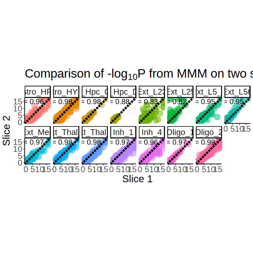
../../_images/analysis_mouse_brain_mouse_brain_MCube_reliability_77_0.png

[ ]:

Sentivity and replicability analysis of MCube

Visium Slice 1

Integrating with RCTD

Cell type deconvolution

Identifying cell-type-specific SVGs using MCube

Integrating with STitch3D

Load in deconvolution results

Identifying cell-type-specific SVGs using MCube

Comparison of the deconvolution results

Comparison of the cell-type-specific SVG results

Detailed comparison of Oligo_2

Visium Slice 2

Integrating with RCTD

Cell type deconvolution

Identifying cell-type-specific SVGs using MCube

Integrating with STitch3D

Load in deconvolution results

Identifying cell-type-specific SVGs using MCube

Comparison of the deconvolution results

Comparison of the cell-type-specific SVG results

Replicability analysis of MCube using the two slices

Comparison of the deconvolution results from RCTD on the two slices

Comparison of the cell-type-specific SVG results on the two slices

Sentivity and replicability analysis of `MCube`

Integrating with `RCTD`

Identifying cell-type-specific SVGs using `MCube`

Integrating with `STitch3D`

Identifying cell-type-specific SVGs using `MCube`

Integrating with `RCTD`

Identifying cell-type-specific SVGs using `MCube`

Integrating with `STitch3D`

Identifying cell-type-specific SVGs using `MCube`

Replicability analysis of `MCube` using the two slices

Comparison of the deconvolution results from `RCTD` on the two slices