Random sample of 20,000 cells from the segmentation results

Typically, analyzing high-resolution spatial transcriptomic (ST) data, such as Xenium data, at the single-cell level requires two preprocessing steps: cell segmentation and cell type annotation, both of which introduce significant uncertainty to the subsequent investigation. Moreover, outcomes from different segmentation and annotation methods can vary a lot, posing a huge challenge for reproducibility.

To demonstrate this, we conduct a comparative experiment on the segmented cells from two different segmentation methods: 10x method and UCS (https://github.com/YangLabHKUST/UCS). We first randomly select 20,000 cells from both methods for analysis.

[1]:

import tifffile
import scanpy as sc
import pandas as pd
import anndata as ad
import numpy as np
import os

data_dir = "/import/home/share/zw/data/breast_cancer"
save_path = "/import/home/share/zw/pql/data/breast_cancer"

Since the new h5ad version, can only be run with pql environment.

[2]:

# scRNA-seq data
adata_sc = sc.read_h5ad(os.path.join(data_dir, "filtered_sc.h5ad"))
adata_sc

[2]:

AnnData object with n_obs × n_vars = 26031 × 307
    obs: 'celltype'
    var: 'gene_ids', 'feature_types', 'genome'

[3]:

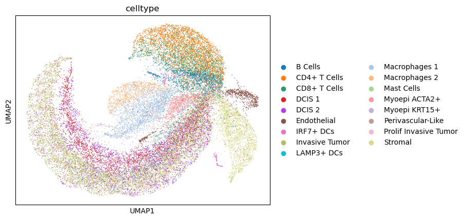
# PCA + UMAP
sc.pp.pca(adata_sc)
sc.pp.neighbors(adata_sc)
sc.tl.umap(adata_sc)

sc.pl.umap(adata_sc, color = "celltype")

/home/zwanghc/anaconda3/envs/pql/lib/python3.11/site-packages/tqdm/auto.py:21: TqdmWarning: IProgress not found. Please update jupyter and ipywidgets. See https://ipywidgets.readthedocs.io/en/stable/user_install.html
  from .autonotebook import tqdm as notebook_tqdm

../../_images/analysis_breast_cancer_breast_cancer_data_5_1.png

[4]:

counts_sc = pd.DataFrame(adata_sc.X.toarray().astype(int), index = adata_sc.obs.index, columns = adata_sc.var_names)
counts_sc.to_csv(os.path.join(save_path, "rawdata", "sc_counts.csv"))

[5]:

adata_sc.obs.to_csv(os.path.join(save_path, "rawdata", "sc_celltypes.csv"))

[6]:

# ST adata with scanvi label and spatial coordinates of mask center
# method = "Cell_10X"
method = "UCS_10X"
adata_st = sc.read_h5ad(os.path.join(data_dir, "paper_data/downstream_xenium_breast_cancer/scVI_output", method, "annotated_adata_st.h5ad"))

[7]:

if not os.path.exists(os.path.join(save_path, method)):
    os.makedirs(os.path.join(save_path, method))
if not os.path.exists(os.path.join(save_path, "rawdata", method)):
    os.makedirs(os.path.join(save_path, "rawdata", method))

[8]:

adata_st

[8]:

AnnData object with n_obs × n_vars = 165734 × 307
    obs: 'tech', '_scvi_batch', '_scvi_labels', 'celltype_scanvi', 'C_scANVI'
    uns: 'C_scANVI_colors', '_scvi_manager_uuid', '_scvi_uuid', 'log1p', 'tech_colors'
    obsm: 'X_mde_scanvi', 'X_scANVI', 'X_scVI', 'X_scVI_mde', 'spatial'
    layers: 'counts'

[9]:

n_spots = adata_st.n_obs
n_samples = 20000
np.random.seed(20240709)
random_indices = np.random.choice(n_spots, size=n_samples, replace=False)
adata_st_subset = adata_st[random_indices]

[10]:

counts = pd.DataFrame(adata_st_subset.layers["counts"].toarray().astype(int),index=adata_st_subset.obs.index,columns=adata_st_subset.var_names)
counts.to_csv(os.path.join(save_path, "rawdata", method, "counts.csv"))

[11]:

adata_st_subset.obsm['spatial']

[11]:

ArrayView([[1678., 1676.],
           [3458., 1343.],
           [ 451., 6580.],
           ...,
           [1318., 2118.],
           [5257., 5898.],
           [1578., 1768.]])

[12]:

coordinates = pd.DataFrame(adata_st_subset.obsm['spatial'].toarray(),index=adata_st_subset.obs.index, columns=["x","y"])
coordinates.to_csv(os.path.join(save_path, "rawdata", method, "coordinates.csv"))

[13]:

scvi_labels = pd.DataFrame(adata_st_subset.obs["C_scANVI"],index=adata_st_subset.obs.index)
scvi_labels.columns = ["celltype"]
scvi_labels.to_csv(os.path.join(save_path, "rawdata", method, "scvi_labels.csv"))

[14]:

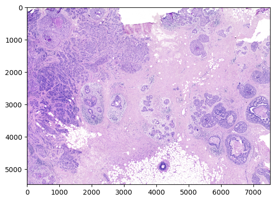
# H&E image
import matplotlib.pyplot as plt
he = tifffile.imread(os.path.join(data_dir, "he.tif"))
plt.imshow(he.transpose(1, 2, 0))

[14]:

<matplotlib.image.AxesImage at 0x7f30c460aa50>

../../_images/analysis_breast_cancer_breast_cancer_data_16_1.png

[15]:

# # Visualization of UCS results (setting method = "UCS_10X")

# import seaborn as sns

# mask = tifffile.imread(os.path.join(data_dir, "UCS_10X.tif"))

# # reset style
# plt.style.use('default')
# plt.figure(figsize=(12, 8))
# plt.ylim(0, mask.shape[0])
# plt.xlim(mask.shape[1], 0)

# # Sorted by cell type
# plot_df = pd.DataFrame(adata_st.obsm['spatial'], columns=['center_x', 'center_y'])
# plot_df['C_scANVI'] = adata_st.obs['C_scANVI'].values
# plot_df = plot_df.sort_values(by='C_scANVI')
# # Selected Endothelial and invasive Tumor / Prolif Invasive Tumor
# # plot_df = plot_df[plot_df['C_scANVI'].isin(["DCIS 1", "DCIS 2", "Invasive Tumor", "Prolif Invasive Tumor", "T Cell & Tumor Hybrid", "Myoepi ACTA2+", "Myoepi KRT15+"])]
# # Change color
# sns.scatterplot(x=plot_df['center_y'], y=plot_df['center_x'],
#                 hue=plot_df['C_scANVI'], s=3 , palette='tab20')
# # Legend outside
# plt.legend(bbox_to_anchor=(-0.32, 0.5), loc='center left', borderaxespad=0., fontsize='x-large', markerscale=10)
# # No axis
# plt.axis('off')
# plt.savefig("/import/home/share/zw/pql/results/breast_cancer/breast_cancer.png", format='png', bbox_inches='tight')
# plt.show()

[16]:

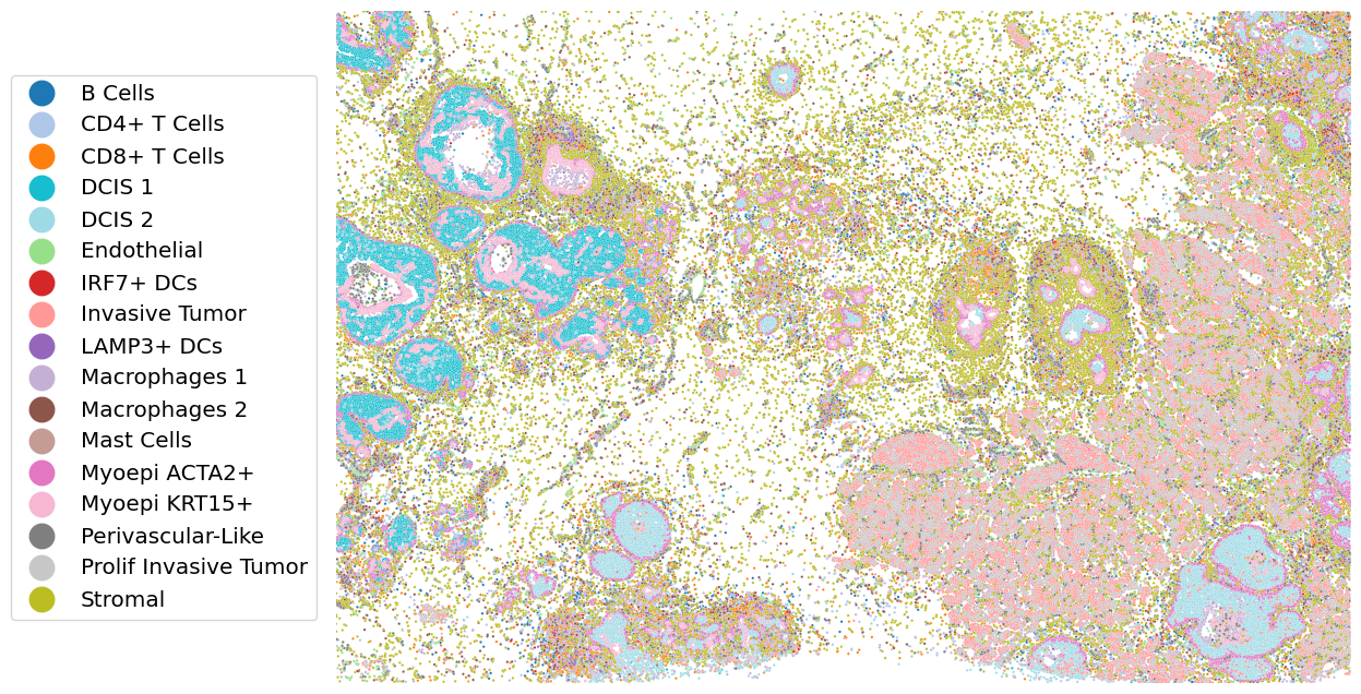
# Visualization of UCS results (setting method = "UCS_10X")

import seaborn as sns

mask = tifffile.imread(os.path.join(data_dir, "UCS_10X.tif"))

# reset style
plt.style.use('default')
plt.figure(figsize=(12, 8))
plt.ylim(0, mask.shape[0])
plt.xlim(mask.shape[1], 0)

# Sorted by cell type
plot_df = pd.DataFrame(adata_st.obsm['spatial'], columns=['center_x', 'center_y'])
plot_df['C_scANVI'] = adata_st.obs['C_scANVI'].values
plot_df = plot_df.sort_values(by='C_scANVI')
# Selected Endothelial and invasive Tumor / Prolif Invasive Tumor
# plot_df = plot_df[plot_df['C_scANVI'].isin(["DCIS 1", "DCIS 2", "Invasive Tumor", "Prolif Invasive Tumor", "T Cell & Tumor Hybrid", "Myoepi ACTA2+", "Myoepi KRT15+"])]

# Customized color palette
all_celltypes = sorted(plot_df['C_scANVI'].unique())
base_palette = sns.color_palette('tab20', len(all_celltypes))
custom_palette = {}
for i, celltype in enumerate(all_celltypes):
    if celltype == "DCIS 1":
        custom_palette[celltype] = sns.color_palette('tab20', 20)[18]
    elif celltype == "DCIS 2":
        custom_palette[celltype] = sns.color_palette('tab20', 20)[19]
    else:
        custom_palette[celltype] = base_palette[i]

# Change color
sns.scatterplot(x=plot_df['center_y'], y=plot_df['center_x'],
                hue=plot_df['C_scANVI'], s=3 , palette=custom_palette)
# Legend outside
plt.legend(bbox_to_anchor=(-0.32, 0.5), loc='center left', borderaxespad=0., fontsize='x-large', markerscale=10)
# No axis
plt.axis('off')
plt.savefig("/import/home/share/zw/pql/results/breast_cancer/breast_cancer_color_scheme.png", format='png', bbox_inches='tight')
plt.savefig("/import/home/share/zw/pql/results/breast_cancer/breast_cancer_color_scheme.pdf", format='pdf', bbox_inches='tight')
plt.show()

../../_images/analysis_breast_cancer_breast_cancer_data_18_0.png

[ ]: