Applying RCTD and MCube to the ST datasets segmented by different methods
[1]:
set.seed(20240709)

library(Matrix)
library(spacexr)
library(MCube)
library(ggplot2)
library(tidyverse)
── Attaching core tidyverse packages ──────────────────────── tidyverse 2.0.0 ──
✔ dplyr     1.1.4     ✔ readr     2.1.5
✔ forcats   1.0.0     ✔ stringr   1.5.1
✔ lubridate 1.9.4     ✔ tibble    3.2.1
✔ purrr     1.0.4     ✔ tidyr     1.3.1
── Conflicts ────────────────────────────────────────── tidyverse_conflicts() ──
✖ tidyr::expand() masks Matrix::expand()
✖ dplyr::filter() masks stats::filter()
✖ dplyr::lag()    masks stats::lag()
✖ tidyr::pack()   masks Matrix::pack()
✖ tidyr::unpack() masks Matrix::unpack()
ℹ Use the conflicted package (<http://conflicted.r-lib.org/>) to force all conflicts to become errors
[2]:
DATA_PATH <- "/import/home/share/zw/pql/data/breast_cancer"
RESULT_PATH <- "/import/home/share/zw/pql/results/breast_cancer"

if (!dir.exists(RESULT_PATH)) {
    dir.create(RESULT_PATH, recursive = TRUE)
}
[3]:
# Load in scRNA-seq reference data

sc_counts <- as.data.frame(readr::read_csv(file.path(DATA_PATH, "rawdata", "sc_counts.csv")))
rownames(sc_counts) <- sc_counts[, 1]
sc_counts[, 1] <- NULL
# head(sc_counts)

sc_celltypes <- read.csv(file.path(DATA_PATH, "rawdata", "sc_celltypes.csv"))
celltypes <- sc_celltypes$celltype
names(celltypes) <- sc_celltypes[, 1]
celltypes <- factor(celltypes, levels = unique(celltypes))

reference <- Reference(t(as.matrix(sc_counts)), celltypes, rowSums(sc_counts), min_UMI = 10)
New names:
• `` -> `...1`
Rows: 26031 Columns: 308
── Column specification ────────────────────────────────────────────────────────
Delimiter: ","
chr   (1): ...1
dbl (307): IL2RG, SNAI1, GLIPR1, OXTR, MYBPC1, MUC6, PDK4, KLRB1, RUNX1, DSP...

ℹ Use `spec()` to retrieve the full column specification for this data.
ℹ Specify the column types or set `show_col_types = FALSE` to quiet this message.
Warning message in check_UMI(nUMI, "Reference", require_2d = T, require_int = require_int, :
“Reference: some nUMI values are less than min_UMI = 10, and these cells will be removed. Optionally, you may lower the min_UMI parameter.”
Cells segmented by the 10x method
Cell type deconvolution using RCTD
[4]:
seg_method <- "Cell_10X"

counts <- as.data.frame(readr::read_csv(
    file.path(DATA_PATH, "rawdata", seg_method, "counts.csv")
))
rownames(counts) <- counts[, 1]
counts[, 1] <- NULL
counts <- as.matrix(counts)
# head(counts)

coordinates <- as.data.frame(readr::read_csv(
    file.path(DATA_PATH, "rawdata", seg_method, "coordinates.csv")
))
rownames(coordinates) <- coordinates[, 1]
coordinates[, 1] <- NULL
coordinates <- as.matrix(coordinates)
# head(coordinates)

# scvi_labels <- as.data.frame(readr::read_csv(
#     file.path(DATA_PATH, "rawdata", seg_method, "scvi_labels.csv")
# ))
# rownames(scvi_labels) <- scvi_labels[, 1]
# scvi_labels <- scvi_labels[, 2]
# # head(scvi_labels)

puck <- SpatialRNA(as.data.frame(coordinates), t(counts), rowSums(counts))
New names:
• `` -> `...1`
Rows: 20000 Columns: 308
── Column specification ────────────────────────────────────────────────────────
Delimiter: ","
dbl (308): ...1, SFRP1, PCLAF, CDC42EP1, LGALSL, CCL5, USP53, IGF1, ESM1, MN...

ℹ Use `spec()` to retrieve the full column specification for this data.
ℹ Specify the column types or set `show_col_types = FALSE` to quiet this message.
New names:
• `` -> `...1`
Rows: 20000 Columns: 3
── Column specification ────────────────────────────────────────────────────────
Delimiter: ","
dbl (3): ...1, x, y

ℹ Use `spec()` to retrieve the full column specification for this data.
ℹ Specify the column types or set `show_col_types = FALSE` to quiet this message.
[5]:
myRCTD <- create.RCTD(
    puck, reference,
    UMI_min = 50, max_cores = 8
)
myRCTD <- run.RCTD(myRCTD, doublet_mode = "doublet")
saveRDS(myRCTD, file.path(RESULT_PATH, seg_method, "myRCTD.rds"))
Begin: process_cell_type_info

process_cell_type_info: number of cells in reference: 25968

process_cell_type_info: number of genes in reference: 307
              Stromal         Macrophages 1     Perivascular-Like
                 2598                  2960                   280
        Myoepi ACTA2+          CD4+ T Cells                DCIS 1
                 1234                  2883                  1861
Prolif Invasive Tumor        Invasive Tumor          CD8+ T Cells
                 1329                  4554                  1839
          Endothelial         Macrophages 2                DCIS 2
                 1053                   760                  2159
              B Cells             IRF7+ DCs            Mast Cells
                 1450                   210                    92
           LAMP3+ DCs         Myoepi KRT15+
                  103                   603
End: process_cell_type_info

create.RCTD: getting regression differentially expressed genes:

get_de_genes: Stromal found DE genes: 33

get_de_genes: Macrophages 1 found DE genes: 36

get_de_genes: Perivascular-Like found DE genes: 36

get_de_genes: Myoepi ACTA2+ found DE genes: 30

get_de_genes: CD4+ T Cells found DE genes: 48

get_de_genes: DCIS 1 found DE genes: 23

get_de_genes: Prolif Invasive Tumor found DE genes: 21

get_de_genes: Invasive Tumor found DE genes: 16

get_de_genes: CD8+ T Cells found DE genes: 44

get_de_genes: Endothelial found DE genes: 41

get_de_genes: Macrophages 2 found DE genes: 33

get_de_genes: DCIS 2 found DE genes: 27

get_de_genes: B Cells found DE genes: 35

get_de_genes: IRF7+ DCs found DE genes: 27

get_de_genes: Mast Cells found DE genes: 19

get_de_genes: LAMP3+ DCs found DE genes: 41

get_de_genes: Myoepi KRT15+ found DE genes: 40

get_de_genes: total DE genes: 275

create.RCTD: getting platform effect normalization differentially expressed genes:

get_de_genes: Stromal found DE genes: 39

get_de_genes: Macrophages 1 found DE genes: 40

get_de_genes: Perivascular-Like found DE genes: 47

get_de_genes: Myoepi ACTA2+ found DE genes: 40

get_de_genes: CD4+ T Cells found DE genes: 51

get_de_genes: DCIS 1 found DE genes: 35

get_de_genes: Prolif Invasive Tumor found DE genes: 40

get_de_genes: Invasive Tumor found DE genes: 30

get_de_genes: CD8+ T Cells found DE genes: 53

get_de_genes: Endothelial found DE genes: 49

get_de_genes: Macrophages 2 found DE genes: 39

get_de_genes: DCIS 2 found DE genes: 36

get_de_genes: B Cells found DE genes: 42

get_de_genes: IRF7+ DCs found DE genes: 30

get_de_genes: Mast Cells found DE genes: 22

get_de_genes: LAMP3+ DCs found DE genes: 51

get_de_genes: Myoepi KRT15+ found DE genes: 56

get_de_genes: total DE genes: 287

fitBulk: decomposing bulk

chooseSigma: using initial Q_mat with sigma =  1

Likelihood value: 238338.905190964

Sigma value:  0.84

Likelihood value: 235350.386294861

Sigma value:  0.69

Likelihood value: 233546.546421314

Sigma value:  0.62

Likelihood value: 233167.74025978

Sigma value:  0.6

Likelihood value: 233125.634474688

Sigma value:  0.59

Likelihood value: 233116.7246218

Sigma value:  0.59
[1] "gather_results: finished 1000"
[1] "gather_results: finished 2000"
[1] "gather_results: finished 3000"
[1] "gather_results: finished 4000"
[1] "gather_results: finished 5000"
[1] "gather_results: finished 6000"
[1] "gather_results: finished 7000"
[1] "gather_results: finished 8000"
[1] "gather_results: finished 9000"
[1] "gather_results: finished 10000"
[1] "gather_results: finished 11000"
[1] "gather_results: finished 12000"
[1] "gather_results: finished 13000"
[1] "gather_results: finished 14000"
[1] "gather_results: finished 15000"
[1] "gather_results: finished 16000"
[1] "gather_results: finished 17000"
[1] "gather_results: finished 18000"
Cell-type-specific SVG identification using MCube
[6]:
seg_method <- "Cell_10X"
myRCTD <- readRDS(file.path(RESULT_PATH, seg_method, "myRCTD.rds"))
[7]:
spot_names <- colnames(myRCTD@spatialRNA@counts)
counts <- t(myRCTD@originalSpatialRNA@counts[, spot_names])
library_sizes_RCTD <- myRCTD@spatialRNA@nUMI
coordinates <- myRCTD@spatialRNA@coords
# sc_counts <- t(myRCTD@reference@counts)
# sc_library_sizes_RCTD <- myRCTD@reference@nUMI
# sc_labels <- myRCTD@reference@cell_types

weights_RCTD <- as.matrix(myRCTD@results$weights)
proportions_RCTD <- weights_RCTD / rowSums(weights_RCTD)

spot_effects_RCTD <- log(rowSums(weights_RCTD))
names(spot_effects_RCTD) <- rownames(weights_RCTD)

reference_RCTD <- t(myRCTD@cell_type_info$info[[1]])
used_for_deconvolution <- rownames(myRCTD@spatialRNA@counts)

# write.csv(as.matrix(counts), file = file.path(DATA_PATH, seg_method, "counts.csv"))
# write.csv(as.matrix(library_sizes_RCTD), file = file.path(DATA_PATH, seg_method, "library_sizes_RCTD.csv"))
# write.csv(coordinates, file = file.path(DATA_PATH, seg_method, "coordinates.csv"))
# write.csv(as.matrix(sc_counts), file = file.path(DATA_PATH, seg_method, "sc_counts.csv"))
# write.csv(as.matrix(sc_library_sizes_RCTD), file = file.path(DATA_PATH, seg_method, "sc_library_sizes_RCTD.csv"))
# write.csv(as.matrix(sc_labels), file = file.path(DATA_PATH, seg_method, "sc_labels.csv"))

# write.csv(weights_RCTD, file = file.path(DATA_PATH, seg_method, "weights_RCTD.csv"))
# write.csv(reference_RCTD, file = file.path(DATA_PATH, seg_method, "reference_RCTD.csv"))
[8]:
mcube_object <- createMCube(
    counts = as.matrix(counts), coordinates = as.matrix(coordinates),
    proportions = proportions_RCTD, library_sizes = library_sizes_RCTD,
    reference = reference_RCTD, used_for_deconvolution = used_for_deconvolution,
    spot_effects = spot_effects_RCTD, platform_effects = NULL,
    project = seg_method
)
mcube_object <- mcubeFitNull(
    mcube_object,
    num_workers = 36, num_threads = 1
)
mcube_object <- mcubeTest(
    mcube_object,
    num_workers = 36, num_threads = 1, shared_memory = TRUE
)
The batch_id is not provided!
All spots are assumed to be from the same batch and share the same gene platform effects.

Select high-abundance cell types to analyze with proportion_threshold = 0.1 and celltype_threshold = 100.

mcubeFilterCellTypes: Cell type(s) Stromal, Macrophages 1, Perivascular-Like, Myoepi ACTA2+, CD4+ T Cells, DCIS 1, Prolif Invasive Tumor, Invasive Tumor, CD8+ T Cells, Endothelial, Macrophages 2, DCIS 2, B Cells, Myoepi KRT15+ pass the threshold.

Cell type(s) IRF7+ DCs, Mast Cells, LAMP3+ DCs has/have less than the minimum celltype_threshold = 100 with proportion_threshold = 0.1.
To include the above cell type(s), please reduce celltype_threshold or proportion_threshold.

Cell type(s) Stromal, Macrophages 1, Perivascular-Like, Myoepi ACTA2+, CD4+ T Cells, DCIS 1, Prolif Invasive Tumor, Invasive Tumor, CD8+ T Cells, Endothelial, Macrophages 2, DCIS 2, B Cells, Myoepi KRT15+ will be analyzed.

Filter out lowly-expressed genes with gene_threshold = 5e-05.

mcubeFilterGenes: 296 genes pass the threshold.

The platform effects are not provided and need to be estimated from data!

Select highly-expressed genes to analyze for each specific cell type with reference_threshold = 0.5.

mcubeFilterGenesCellType: Select 59 genes to analyze for Stromal.

mcubeFilterGenesCellType: Select 62 genes to analyze for Macrophages 1.

mcubeFilterGenesCellType: Select 60 genes to analyze for Perivascular-Like.

mcubeFilterGenesCellType: Select 59 genes to analyze for Myoepi ACTA2+.

mcubeFilterGenesCellType: Select 58 genes to analyze for CD4+ T Cells.

mcubeFilterGenesCellType: Select 59 genes to analyze for DCIS 1.

mcubeFilterGenesCellType: Select 61 genes to analyze for Prolif Invasive Tumor.

mcubeFilterGenesCellType: Select 53 genes to analyze for Invasive Tumor.

mcubeFilterGenesCellType: Select 60 genes to analyze for CD8+ T Cells.

mcubeFilterGenesCellType: Select 71 genes to analyze for Endothelial.

mcubeFilterGenesCellType: Select 45 genes to analyze for Macrophages 2.

mcubeFilterGenesCellType: Select 61 genes to analyze for DCIS 2.

mcubeFilterGenesCellType: Select 64 genes to analyze for B Cells.

mcubeFilterGenesCellType: Select 80 genes to analyze for Myoepi KRT15+.

Preprocessed data description: 18312 spots and 17 cell types in total. 18302 spots, 295 genes, and 14 cell type(s) to analyze.

Number of physical cores: 40.

Number of workers: 36.

Number of thread(s) on BLAS per worker: 1.

mcubeKernel: length_scale is set as 0.0174020195267825 for the Gaussian kernel.

mcubeKernel: length_scale is set as 0.0246101720274573 for the Gaussian kernel.

mcubeKernel: length_scale is set as 0.0174020195267825 for the Gaussian_transformed kernel.

mcubeKernel: length_scale is set as 0.0246101720274573 for the Gaussian_transformed kernel.

Number of physical cores: 40.

Number of workers: 36.

Number of thread(s) on BLAS per worker: 1.
[9]:
saveRDS(mcube_object,
    file = file.path(
        RESULT_PATH, seg_method,
        paste0(
            "mcube_object",
            ".rds"
        )
    )
)

pvalues_10x <- mcube_object@pvalues
saveRDS(mcube_object@pvalues,
    file = file.path(
        RESULT_PATH, seg_method,
        paste0(
            "mcube_pvalues",
            ".rds"
        )
    )
)
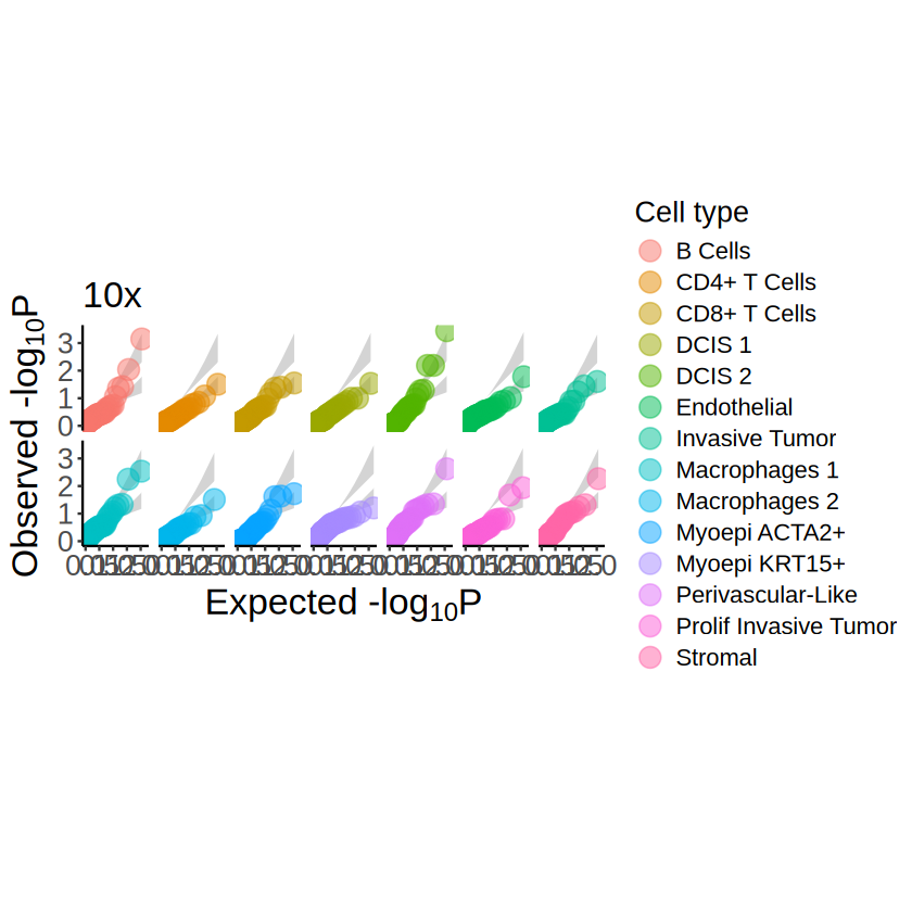
Negative control
[10]:
shuffle_idx <- sample(1:nrow(mcube_object@coordinates), nrow(mcube_object@coordinates))
mcube_object_null <- mcube_object
mcube_object_null@coordinates <- mcube_object@coordinates[shuffle_idx, ]
rownames(mcube_object_null@coordinates) <- rownames(mcube_object@coordinates)
mcube_object_null <- mcubeTest(
    mcube_object_null,
    num_workers = 36, num_threads = 1, shared_memory = TRUE
)

p <- mcubePlotPvalues(
    mcube_object_null@pvalues, "combined_pvalue",
    minus_log10p_max = 4, nrow = 2, under_null = TRUE
)
p <- p +
    labs(title = "10x") +
    theme(
        text = element_text(size = 16),
        plot.title = element_text(size = 20),
        axis.title = element_text(size = 20),
        axis.text.x = element_text(size = 16),
        axis.text.y = element_text(size = 16)
    )
p
ggsave(
    filename = file.path(
        RESULT_PATH, seg_method,
        paste0("pvalues_qqplot_null.pdf")),
    plot = p, width = 12, height = 6
)

rm(mcube_object_null)
mcubeKernel: length_scale is set as 0.0174020195267825 for the Gaussian kernel.

mcubeKernel: length_scale is set as 0.0246101720274573 for the Gaussian kernel.

mcubeKernel: length_scale is set as 0.0174020195267825 for the Gaussian_transformed kernel.

mcubeKernel: length_scale is set as 0.0246101720274573 for the Gaussian_transformed kernel.

Number of physical cores: 40.

Number of workers: 36.

Number of thread(s) on BLAS per worker: 1.
Cells segmented by UCS
Cell type deconvolution using RCTD
[11]:
seg_method <- "UCS_10X"

counts <- as.data.frame(readr::read_csv(
    file.path(DATA_PATH, "rawdata", seg_method, "counts.csv")
))
rownames(counts) <- counts[, 1]
counts[, 1] <- NULL
counts <- as.matrix(counts)
# head(counts)

coordinates <- as.data.frame(readr::read_csv(
    file.path(DATA_PATH, "rawdata", seg_method, "coordinates.csv")
))
rownames(coordinates) <- coordinates[, 1]
coordinates[, 1] <- NULL
coordinates <- as.matrix(coordinates)
# head(coordinates)

# scvi_labels <- as.data.frame(readr::read_csv(
#     file.path(DATA_PATH, "rawdata", seg_method, "scvi_labels.csv")
# ))
# rownames(scvi_labels) <- scvi_labels[, 1]
# scvi_labels <- scvi_labels[, 2]
# # head(scvi_labels)

puck <- SpatialRNA(as.data.frame(coordinates), t(counts), rowSums(counts))
New names:
• `` -> `...1`
Rows: 20000 Columns: 308
── Column specification ────────────────────────────────────────────────────────
Delimiter: ","
dbl (308): ...1, IL2RG, SNAI1, GLIPR1, OXTR, MYBPC1, MUC6, PDK4, KLRB1, RUNX...

ℹ Use `spec()` to retrieve the full column specification for this data.
ℹ Specify the column types or set `show_col_types = FALSE` to quiet this message.
New names:
• `` -> `...1`
Rows: 20000 Columns: 3
── Column specification ────────────────────────────────────────────────────────
Delimiter: ","
dbl (3): ...1, x, y

ℹ Use `spec()` to retrieve the full column specification for this data.
ℹ Specify the column types or set `show_col_types = FALSE` to quiet this message.
[12]:
myRCTD <- create.RCTD(
    puck, reference,
    UMI_min = 50, max_cores = 8
)
myRCTD <- run.RCTD(myRCTD, doublet_mode = "doublet")
saveRDS(myRCTD, file.path(RESULT_PATH, seg_method, "myRCTD.rds"))
Begin: process_cell_type_info

process_cell_type_info: number of cells in reference: 25968

process_cell_type_info: number of genes in reference: 307
              Stromal         Macrophages 1     Perivascular-Like
                 2598                  2960                   280
        Myoepi ACTA2+          CD4+ T Cells                DCIS 1
                 1234                  2883                  1861
Prolif Invasive Tumor        Invasive Tumor          CD8+ T Cells
                 1329                  4554                  1839
          Endothelial         Macrophages 2                DCIS 2
                 1053                   760                  2159
              B Cells             IRF7+ DCs            Mast Cells
                 1450                   210                    92
           LAMP3+ DCs         Myoepi KRT15+
                  103                   603
End: process_cell_type_info

create.RCTD: getting regression differentially expressed genes:

get_de_genes: Stromal found DE genes: 33

get_de_genes: Macrophages 1 found DE genes: 36

get_de_genes: Perivascular-Like found DE genes: 36

get_de_genes: Myoepi ACTA2+ found DE genes: 30

get_de_genes: CD4+ T Cells found DE genes: 48

get_de_genes: DCIS 1 found DE genes: 23

get_de_genes: Prolif Invasive Tumor found DE genes: 21

get_de_genes: Invasive Tumor found DE genes: 16

get_de_genes: CD8+ T Cells found DE genes: 44

get_de_genes: Endothelial found DE genes: 41

get_de_genes: Macrophages 2 found DE genes: 33

get_de_genes: DCIS 2 found DE genes: 27

get_de_genes: B Cells found DE genes: 35

get_de_genes: IRF7+ DCs found DE genes: 27

get_de_genes: Mast Cells found DE genes: 19

get_de_genes: LAMP3+ DCs found DE genes: 41

get_de_genes: Myoepi KRT15+ found DE genes: 40

get_de_genes: total DE genes: 275

create.RCTD: getting platform effect normalization differentially expressed genes:

get_de_genes: Stromal found DE genes: 39

get_de_genes: Macrophages 1 found DE genes: 40

get_de_genes: Perivascular-Like found DE genes: 47

get_de_genes: Myoepi ACTA2+ found DE genes: 40

get_de_genes: CD4+ T Cells found DE genes: 51

get_de_genes: DCIS 1 found DE genes: 35

get_de_genes: Prolif Invasive Tumor found DE genes: 40

get_de_genes: Invasive Tumor found DE genes: 30

get_de_genes: CD8+ T Cells found DE genes: 53

get_de_genes: Endothelial found DE genes: 49

get_de_genes: Macrophages 2 found DE genes: 39

get_de_genes: DCIS 2 found DE genes: 36

get_de_genes: B Cells found DE genes: 42

get_de_genes: IRF7+ DCs found DE genes: 30

get_de_genes: Mast Cells found DE genes: 22

get_de_genes: LAMP3+ DCs found DE genes: 51

get_de_genes: Myoepi KRT15+ found DE genes: 56

get_de_genes: total DE genes: 287

fitBulk: decomposing bulk

chooseSigma: using initial Q_mat with sigma =  1

Likelihood value: 215701.707758942

Sigma value:  0.84

Likelihood value: 212004.921428186

Sigma value:  0.69

Likelihood value: 209239.718715138

Sigma value:  0.61

Likelihood value: 208180.814538632

Sigma value:  0.53

Likelihood value: 207520.002104391

Sigma value:  0.49

Likelihood value: 207372.187267782

Sigma value:  0.47

Likelihood value: 207350.233963885

Sigma value:  0.47
[1] "gather_results: finished 1000"
[1] "gather_results: finished 2000"
[1] "gather_results: finished 3000"
[1] "gather_results: finished 4000"
[1] "gather_results: finished 5000"
[1] "gather_results: finished 6000"
[1] "gather_results: finished 7000"
[1] "gather_results: finished 8000"
[1] "gather_results: finished 9000"
[1] "gather_results: finished 10000"
[1] "gather_results: finished 11000"
[1] "gather_results: finished 12000"
[1] "gather_results: finished 13000"
[1] "gather_results: finished 14000"
[1] "gather_results: finished 15000"
[1] "gather_results: finished 16000"
[1] "gather_results: finished 17000"
Cell-type-specific SVG identification using MCube
[13]:
seg_method <- "UCS_10X"
myRCTD <- readRDS(file.path(RESULT_PATH, seg_method, "myRCTD.rds"))
[14]:
spot_names <- colnames(myRCTD@spatialRNA@counts)
counts <- t(myRCTD@originalSpatialRNA@counts[, spot_names])
library_sizes_RCTD <- myRCTD@spatialRNA@nUMI
coordinates <- myRCTD@spatialRNA@coords
# sc_counts <- t(myRCTD@reference@counts)
# sc_library_sizes_RCTD <- myRCTD@reference@nUMI
# sc_labels <- myRCTD@reference@cell_types

weights_RCTD <- as.matrix(myRCTD@results$weights)
proportions_RCTD <- weights_RCTD / rowSums(weights_RCTD)

spot_effects_RCTD <- log(rowSums(weights_RCTD))
names(spot_effects_RCTD) <- rownames(weights_RCTD)

reference_RCTD <- t(myRCTD@cell_type_info$info[[1]])
used_for_deconvolution <- rownames(myRCTD@spatialRNA@counts)

# write.csv(as.matrix(counts), file = file.path(DATA_PATH, seg_method, "counts.csv"))
# write.csv(as.matrix(library_sizes_RCTD), file = file.path(DATA_PATH, seg_method, "library_sizes_RCTD.csv"))
# write.csv(coordinates, file = file.path(DATA_PATH, seg_method, "coordinates.csv"))
# write.csv(as.matrix(sc_counts), file = file.path(DATA_PATH, seg_method, "sc_counts.csv"))
# write.csv(as.matrix(sc_library_sizes_RCTD), file = file.path(DATA_PATH, seg_method, "sc_library_sizes_RCTD.csv"))
# write.csv(as.matrix(sc_labels), file = file.path(DATA_PATH, seg_method, "sc_labels.csv"))

# write.csv(weights_RCTD, file = file.path(DATA_PATH, seg_method, "weights_RCTD.csv"))
# write.csv(reference_RCTD, file = file.path(DATA_PATH, seg_method, "reference_RCTD.csv"))
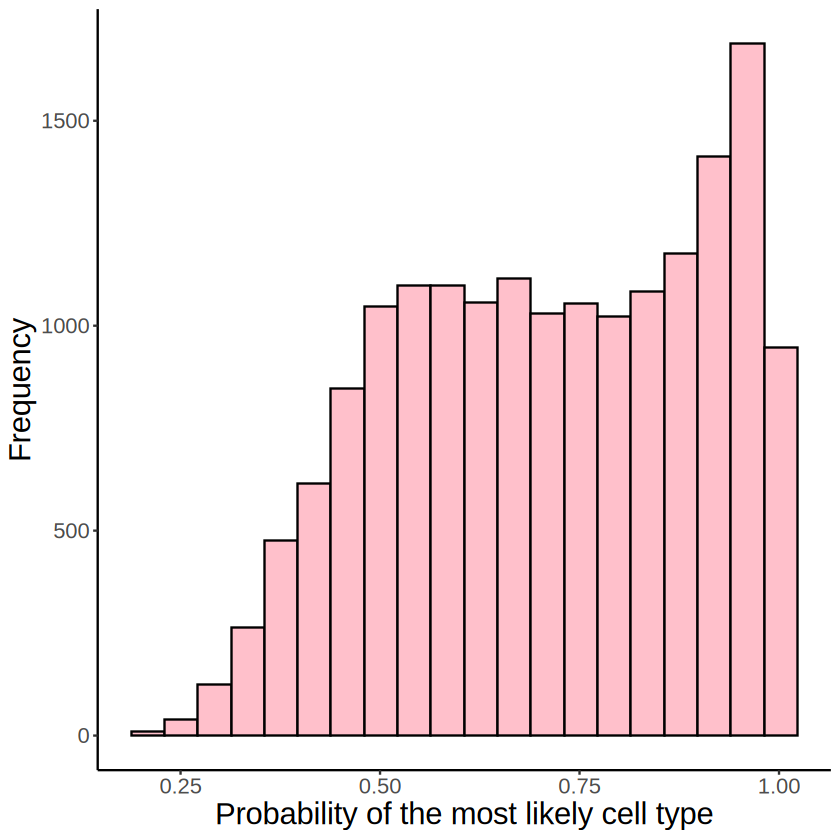
[15]:
p <- ggplot(NULL, aes(apply(proportions_RCTD, 1, max))) +
    geom_histogram(bins = 20, fill = "pink", color = "black") +
    theme_classic() +
    labs(
        title = NULL,
        x = "Probability of the most likely cell type",
        y = "Frequency"
    ) +
    theme(
        axis.title = element_text(size = 18),
        text = element_text(size = 16),
    )
p
ggsave(
    file = file.path(RESULT_PATH, seg_method, "hist_most_likely_celltype.pdf"),
    plot = p, width = 5, height = 4
)
[16]:
threshold_seq <- seq(from = 0.75, to = 0.95, by = 0.05)
credible_sets <- matrix(NA, nrow = nrow(proportions_RCTD), ncol = length(threshold_seq))
colnames(credible_sets) <- as.character(threshold_seq)
for (i in 1:length(threshold_seq)) {
    credible_sets[, i] <- apply(
        proportions_RCTD,
        MARGIN = 1,
        FUN = getCredibleSetSize,
        threshold = threshold_seq[i]
    )
}
credible_sets <- as.data.frame(credible_sets)
credible_sets$spot <- rownames(proportions_RCTD)
credible_sets_long <- tidyr::pivot_longer(
  credible_sets,
  cols = -spot,
  names_to = "threshold",
  values_to = "credible_set_size"
)

p <- ggplot(data = credible_sets_long,
aes(x = threshold, y = credible_set_size, color = threshold, fill = threshold)) +
    geom_violin(adjust = 5) +
    theme_classic() +
    scale_y_continuous(
        limits = c(1, NA),
        breaks = scales::pretty_breaks(n = 4)(range(credible_sets_long$credible_set_size))
    ) +
    labs(
        title = NULL,
        x = "Threshold",
        y = "Credible set size"
    ) +
    theme(
        axis.title = element_text(size = 18),
        text = element_text(size = 16),
        legend.position = "none"
    )
p
ggsave(
    file = file.path(RESULT_PATH, seg_method, "credible_set_size.pdf"),
    plot = p, width = 5, height = 4
)

[17]:
mcube_object <- createMCube(
    counts = as.matrix(counts), coordinates = as.matrix(coordinates),
    proportions = proportions_RCTD, library_sizes = library_sizes_RCTD,
    reference = reference_RCTD, used_for_deconvolution = used_for_deconvolution,
    spot_effects = spot_effects_RCTD, platform_effects = NULL,
    project = seg_method
)
mcube_object <- mcubeFitNull(
    mcube_object,
    num_workers = 36, num_threads = 1
)
mcube_object <- mcubeTest(
    mcube_object,
    num_workers = 36, num_threads = 1, shared_memory = TRUE
)
The batch_id is not provided!
All spots are assumed to be from the same batch and share the same gene platform effects.

Select high-abundance cell types to analyze with proportion_threshold = 0.1 and celltype_threshold = 100.

mcubeFilterCellTypes: Cell type(s) Stromal, Macrophages 1, Perivascular-Like, Myoepi ACTA2+, CD4+ T Cells, DCIS 1, Prolif Invasive Tumor, Invasive Tumor, CD8+ T Cells, Endothelial, Macrophages 2, DCIS 2, B Cells, Myoepi KRT15+ pass the threshold.

Cell type(s) IRF7+ DCs, Mast Cells, LAMP3+ DCs has/have less than the minimum celltype_threshold = 100 with proportion_threshold = 0.1.
To include the above cell type(s), please reduce celltype_threshold or proportion_threshold.

Cell type(s) Stromal, Macrophages 1, Perivascular-Like, Myoepi ACTA2+, CD4+ T Cells, DCIS 1, Prolif Invasive Tumor, Invasive Tumor, CD8+ T Cells, Endothelial, Macrophages 2, DCIS 2, B Cells, Myoepi KRT15+ will be analyzed.

Filter out lowly-expressed genes with gene_threshold = 5e-05.

mcubeFilterGenes: 294 genes pass the threshold.

The platform effects are not provided and need to be estimated from data!

Select highly-expressed genes to analyze for each specific cell type with reference_threshold = 0.5.

mcubeFilterGenesCellType: Select 58 genes to analyze for Stromal.

mcubeFilterGenesCellType: Select 62 genes to analyze for Macrophages 1.

mcubeFilterGenesCellType: Select 60 genes to analyze for Perivascular-Like.

mcubeFilterGenesCellType: Select 59 genes to analyze for Myoepi ACTA2+.

mcubeFilterGenesCellType: Select 58 genes to analyze for CD4+ T Cells.

mcubeFilterGenesCellType: Select 59 genes to analyze for DCIS 1.

mcubeFilterGenesCellType: Select 61 genes to analyze for Prolif Invasive Tumor.

mcubeFilterGenesCellType: Select 52 genes to analyze for Invasive Tumor.

mcubeFilterGenesCellType: Select 60 genes to analyze for CD8+ T Cells.

mcubeFilterGenesCellType: Select 70 genes to analyze for Endothelial.

mcubeFilterGenesCellType: Select 44 genes to analyze for Macrophages 2.

mcubeFilterGenesCellType: Select 61 genes to analyze for DCIS 2.

mcubeFilterGenesCellType: Select 67 genes to analyze for B Cells.

mcubeFilterGenesCellType: Select 79 genes to analyze for Myoepi KRT15+.

Preprocessed data description: 17201 spots and 17 cell types in total. 17169 spots, 293 genes, and 14 cell type(s) to analyze.

Number of physical cores: 40.

Number of workers: 36.

Number of thread(s) on BLAS per worker: 1.

mcubeKernel: length_scale is set as 0.0166496112180841 for the Gaussian kernel.

mcubeKernel: length_scale is set as 0.0235461059928537 for the Gaussian kernel.

mcubeKernel: length_scale is set as 0.0166496112180841 for the Gaussian_transformed kernel.

mcubeKernel: length_scale is set as 0.0235461059928537 for the Gaussian_transformed kernel.

Number of physical cores: 40.

Number of workers: 36.

Number of thread(s) on BLAS per worker: 1.
[18]:
saveRDS(mcube_object,
    file = file.path(
        RESULT_PATH, seg_method,
        paste0(
            "mcube_object",
            ".rds"
        )
    )
)

pvalues_UCS <- mcube_object@pvalues
saveRDS(pvalues_UCS,
    file = file.path(
        RESULT_PATH, seg_method,
        paste0(
            "mcube_pvalues",
            ".rds"
        )
    )
)
Negative control
[19]:
shuffle_idx <- sample(1:nrow(mcube_object@coordinates), nrow(mcube_object@coordinates))
mcube_object_null <- mcube_object
mcube_object_null@coordinates <- mcube_object@coordinates[shuffle_idx, ]
rownames(mcube_object_null@coordinates) <- rownames(mcube_object@coordinates)
mcube_object_null <- mcubeTest(
    mcube_object_null,
    num_workers = 36, num_threads = 1, shared_memory = TRUE
)

p <- mcubePlotPvalues(
    mcube_object_null@pvalues, "combined_pvalue",
    minus_log10p_max = 4, nrow = 2, under_null = TRUE
)
p <- p +
    labs(title = "UCS") +
    theme(
        text = element_text(size = 16),
        plot.title = element_text(size = 20),
        axis.title = element_text(size = 20),
        axis.text.x = element_text(size = 16),
        axis.text.y = element_text(size = 16)
    )
p
ggsave(
    filename = file.path(
        RESULT_PATH, seg_method,
        paste0("pvalues_qqplot_null.pdf")),
    plot = p, width = 12, height = 6
)

rm(mcube_object_null)
mcubeKernel: length_scale is set as 0.0166496112180841 for the Gaussian kernel.

mcubeKernel: length_scale is set as 0.0235461059928537 for the Gaussian kernel.

mcubeKernel: length_scale is set as 0.0166496112180841 for the Gaussian_transformed kernel.

mcubeKernel: length_scale is set as 0.0235461059928537 for the Gaussian_transformed kernel.

Number of physical cores: 40.

Number of workers: 36.

Number of thread(s) on BLAS per worker: 1.

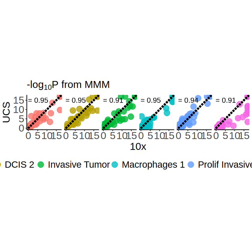
Comparsion of the cell-type-specific SVG identification results
[20]:
pvalues_10x <- readRDS(
    file = file.path(
        RESULT_PATH, "Cell_10X",
        paste0(
            "mcube_pvalues",
            ".rds"
        )
    )
)
pvalues_UCS <- readRDS(
    file = file.path(
        RESULT_PATH, "UCS_10X",
        paste0(
            "mcube_pvalues",
            ".rds"
        )
    )
)
[21]:
log10p_lim <- 17 # 5.55e-17
pvalues_10x_long <- do.call(
    rbind,
    lapply(
        names(pvalues_10x),
        FUN = function(x) {
            data.frame(
                celltype = x,
                gene = rownames(pvalues_10x[[x]]),
                pvalue = pvalues_10x[[x]][, "combined_pvalue"]
            )
        }
    )
)
pvalues_10x_long$minus_log10_pvalue <- -log10(pvalues_10x_long$pvalue)
pvalues_10x_long$minus_log10_pvalue[pvalues_10x_long$minus_log10_pvalue > log10p_lim] <- log10p_lim

pvalues_UCS_long <- do.call(
    rbind,
    lapply(
        names(pvalues_UCS),
        FUN = function(x) {
            data.frame(
                celltype = x,
                gene = rownames(pvalues_UCS[[x]]),
                pvalue = pvalues_UCS[[x]][, "combined_pvalue"]
            )
        }
    )
)
pvalues_UCS_long$minus_log10_pvalue <- -log10(pvalues_UCS_long$pvalue)
pvalues_UCS_long$minus_log10_pvalue[pvalues_UCS_long$minus_log10_pvalue > log10p_lim] <- log10p_lim

pvalues_all <- merge(
    pvalues_10x_long,
    pvalues_UCS_long,
    by = c("celltype", "gene"),
    suffixes = c("_10x", "_UCS")
)
dim(pvalues_all)
head(pvalues_all)
- 799
- 6
| celltype | gene | pvalue_10x | minus_log10_pvalue_10x | pvalue_UCS | minus_log10_pvalue_UCS | |
|---|---|---|---|---|---|---|
| <chr> | <chr> | <dbl> | <dbl> | <dbl> | <dbl> | |
| 1 | B Cells | ANKRD28 | 1.199796e-01 | 0.92089242 | 1.773733e-01 | 0.7511117 |
| 2 | B Cells | BANK1 | 3.319030e-29 | 17.00000000 | 2.938843e-31 | 17.0000000 |
| 3 | B Cells | BASP1 | 2.478064e-01 | 0.60588749 | 6.127142e-02 | 1.2127421 |
| 4 | B Cells | C2orf42 | 3.381138e-01 | 0.47093714 | 4.458187e-01 | 0.3508417 |
| 5 | B Cells | CCDC6 | 8.267835e-01 | 0.08260818 | 6.341681e-01 | 0.1977956 |
| 6 | B Cells | CCPG1 | 1.573644e-04 | 3.80309362 | 3.320999e-03 | 2.4787312 |
[22]:
correlations <- pvalues_all %>%
    group_by(celltype) %>%
    summarize(
        correlation = cor(minus_log10_pvalue_10x, minus_log10_pvalue_UCS, method = "pearson")
    )
[23]:
# major_celltypes <- mcube_object@celltype_test
major_celltypes <- c(
    "Invasive Tumor", "Stromal", "DCIS 1", "DCIS 2",
    "Prolif Invasive Tumor", "Macrophages 1"
)
pvalues_all_major_celltype <- pvalues_all[pvalues_all$celltype %in% major_celltypes, ]
pvalues_all_major_celltype$celltype <- factor(
    pvalues_all_major_celltype$celltype,
    levels = sort(major_celltypes)
)
correlations_major_celltype <- correlations[correlations$celltype %in% major_celltypes, ]

p <- ggplot(
    # pvalues_all,
    pvalues_all_major_celltype,
    aes(x = minus_log10_pvalue_10x, y = minus_log10_pvalue_UCS)
) +geom_point(aes(color = celltype), size = 5, alpha = 0.8) +
        geom_abline(
            intercept = 0, slope = 1,
            linetype = "longdash", linewidth = 1.5
        ) + geom_text(
            data = correlations_major_celltype,
            mapping = aes(
                x = 4, y = 15,
                label = paste("r =", round(correlation, 2))
            ),
            size = 5
        ) +
    scale_x_continuous(limits = c(0, log10p_lim), oob = scales::oob_squish) +
    scale_y_continuous(limits = c(0, log10p_lim), oob = scales::oob_squish) +
    coord_fixed(ratio = 1) +
    facet_wrap(~ celltype, nrow = 1) +
    theme_classic() +
    labs(
        x = "10x", y = "UCS",
        title = expression(paste("-log"[10], plain(P), " from MMM"))
    ) +
    guides(color = guide_legend(nrow = 1)) +
    theme(
        plot.title = element_text(size = 20),
        axis.title = element_text(size = 20),
        axis.text.x = element_text(size = 20),
        axis.text.y = element_text(size = 20),
        strip.text = element_blank(),
        legend.title = element_blank(),
        legend.text = element_text(size = 18),
        legend.position = "bottom"
    )
ggsave(
    filename = file.path(
        RESULT_PATH, paste0("MMM_seg_comparison_oob_squish_", log10p_lim, ".pdf")
    ),
    plot = p, width = 12, height = 4
)
p
Visualization of the identified cell-type-specific SVGs
We then visualize the cell-type-specific SVG identification results of the ST dataset segmented by UCS.
[24]:
# mcube_object <- readRDS(
#     file = file.path(
#         RESULT_PATH, "UCS_10X",
#         paste0(
#             "mcube_object",
#             ".rds"
#         )
#     )
# )

sig_genes <- mcubeGetSigGenes(mcube_object@pvalues)
mcubeGetSigGenes: Set adjust_method as BH and alpha as 0.05.
[25]:
# Load in H&E image
library(tiff)
library(grid)
library(nara)
he_image <- readTIFF(file.path(DATA_PATH, "he.tif"), native = TRUE)
he_image <- nr_flipv(he_image)
he_image <- nr_fliph(he_image)
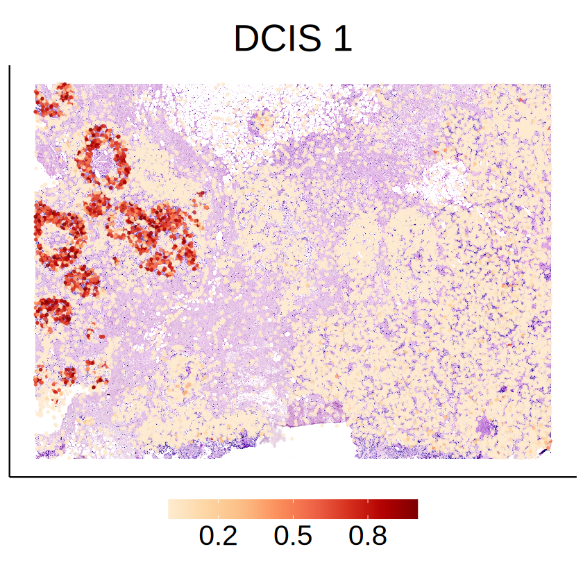
Cell type DCIS 1
[26]:
celltype <- "DCIS 1"
[27]:
# Cell type proportion
plot_df <- data.frame(
    x = mcube_object@coordinates[, 2],
    y = mcube_object@coordinates[, 1],
    prop = mcube_object@proportions[, celltype]
)
plot_df <- plot_df[plot_df$prop > 0, , drop = FALSE]

p <- ggplot(data = plot_df, aes(x = x, y = y)) +
annotation_raster(
    he_image,
    xmin = -max(mcube_object@coordinates[, 2]), xmax = 0,
    ymin = 0, ymax = max(mcube_object@coordinates[, 1])
) +
    geom_point(aes(color = prop), size = 0.5, alpha = 0.8) +
    scale_x_continuous(transform = "reverse") +
    scale_colour_gradientn(
        name = NULL,
        colors = pals::brewer.orrd(22)[3:22],
        breaks = c(0.2,0.5,0.8)) +
    guides(color = guide_colorbar(barwidth = 15)) +
    coord_fixed(ratio = 1) +
    labs(title = celltype, x = NULL, y = NULL) +
    theme_classic() +
    theme(
        text = element_text(family = "Helvetica"),
        plot.title = element_text(size = 32, hjust = 0.5),
        axis.title = element_blank(),
        axis.ticks = element_blank(),
        axis.text = element_blank(),
        legend.position = "bottom",
        legend.title = element_blank(),
        legend.text = element_text(size = 24),
    )
ggsave(
    filename = file.path(RESULT_PATH, paste0(celltype, "_proportion.png")),
    plot = p, width = 5, height = 5
)
p
[28]:
# Cell-type-specific SVGS
write.table(
    rownames(sig_genes[[celltype]]),
    file = file.path(
        RESULT_PATH,
        paste0(celltype, "_SVG", ".txt")
    ),
    quote = FALSE, row.names = FALSE, col.names = FALSE
)
head(sig_genes[[celltype]])
| pvalue | adjusted_pvalue | |
|---|---|---|
| <dbl> | <dbl> | |
| SERPINA3 | 6.424971e-165 | 3.790733e-163 |
| ESR1 | 3.319651e-70 | 9.792971e-69 |
| SCD | 5.330236e-57 | 1.048280e-55 |
| TACSTD2 | 2.012262e-51 | 2.968087e-50 |
| ERBB2 | 1.870009e-50 | 2.206611e-49 |
| USP53 | 2.223889e-40 | 2.186824e-39 |
[29]:
demo_genes <- c("SERPINA3", "ESR1", "SCD")
for (gene in demo_genes) {
    pair_name <- paste(celltype, gene, sep = "_")
    null_model_results <- mcube_object@null_models[[pair_name]]
    spots <- null_model_results$spots
    u <- null_model_results$u[spots, celltype]
    rel_expr_level <- factor(ifelse(u >= 0, "Higher", "Lower"))
    plot_df <- data.frame(
        x = mcube_object@coordinates[spots, 2],
        y = mcube_object@coordinates[spots, 1],
        rel_expr_level = rel_expr_level
    )

    p <- ggplot(data = plot_df, aes(x = x, y = y)) +
        annotation_raster(
            he_image,
            xmin = -max(mcube_object@coordinates[, 2]), xmax = 0,
            ymin = 0, ymax = max(mcube_object@coordinates[, 1])
        ) +
        geom_point(aes(color = rel_expr_level), size = 0.5, alpha = 0.95) +
        scale_color_manual(name = "Level", values = c(`Lower` = "#32CD32", `Higher` = "#FF69B4")) +
        scale_x_continuous(transform = "reverse") +
        guides(color = guide_legend(override.aes = list(size = 5))) +
        coord_fixed(ratio = 1) +
        labs(title = gene, x = NULL, y = NULL) +
        theme_classic() +
        theme(
            text = element_text(family = "Helvetica"),
            plot.title = element_text(face = "italic", size = 32, hjust = 0.5),
            axis.title = element_blank(),
            axis.text = element_blank(),
            axis.ticks = element_blank(),
            legend.position = "bottom",
            legend.title = element_blank(),
            legend.text = element_text(size = 28)
        )
    ggsave(
        filename = file.path(RESULT_PATH, paste0(celltype, "_", gene, ".png")),
        plot = p, width = 5, height = 5
    )
}
p

Cell type DCIS 2
[30]:
celltype <- "DCIS 2"
[31]:
# Cell type proportion
plot_df <- data.frame(
    x = mcube_object@coordinates[, 2],
    y = mcube_object@coordinates[, 1],
    prop = mcube_object@proportions[, celltype]
)
plot_df <- plot_df[plot_df$prop > 0, , drop = FALSE]

p <- ggplot(data = plot_df, aes(x = x, y = y)) +
annotation_raster(
    he_image,
    xmin = -max(mcube_object@coordinates[, 2]), xmax = 0,
    ymin = 0, ymax = max(mcube_object@coordinates[, 1])
) +
    geom_point(aes(color = prop), size = 0.5, alpha = 0.8) +
    scale_x_continuous(transform = "reverse") +
    scale_colour_gradientn(
        name = NULL,
        colors = pals::brewer.orrd(22)[3:22],
        breaks = c(0.2,0.5,0.8)) +
    guides(color = guide_colorbar(barwidth = 15)) +
    coord_fixed(ratio = 1) +
    labs(title = celltype, x = NULL, y = NULL) +
    theme_classic() +
    theme(
        text = element_text(family = "Helvetica"),
        plot.title = element_text(size = 32, hjust = 0.5),
        axis.title = element_blank(),
        axis.ticks = element_blank(),
        axis.text = element_blank(),
        legend.position = "bottom",
        legend.title = element_blank(),
        legend.text = element_text(size = 24),
    )
ggsave(
    filename = file.path(RESULT_PATH, paste0(celltype, "_proportion.png")),
    plot = p, width = 5, height = 5
)
p

[32]:
# Cell-type-specific SVGS
write.table(
    rownames(sig_genes[[celltype]]),
    file = file.path(
        RESULT_PATH,
        paste0(celltype, "_SVG", ".txt")
    ),
    quote = FALSE, row.names = FALSE, col.names = FALSE
)
head(sig_genes[[celltype]])
| pvalue | adjusted_pvalue | |
|---|---|---|
| <dbl> | <dbl> | |
| SERPINA3 | 1.315390e-255 | 7.760800e-254 |
| CEACAM6 | 7.774769e-235 | 2.293557e-233 |
| SCD | 3.980345e-207 | 7.828011e-206 |
| TENT5C | 1.150485e-183 | 1.696965e-182 |
| KRT7 | 2.338823e-147 | 2.759812e-146 |
| ERBB2 | 3.040227e-140 | 2.989556e-139 |
[33]:
demo_genes <- c("CEACAM6", "SERPINA3", "KRT7")
for (gene in demo_genes) {
    pair_name <- paste(celltype, gene, sep = "_")
    null_model_results <- mcube_object@null_models[[pair_name]]
    spots <- null_model_results$spots
    u <- null_model_results$u[spots, celltype]
    rel_expr_level <- factor(ifelse(u >= 0, "Higher", "Lower"))
    plot_df <- data.frame(
        x = mcube_object@coordinates[spots, 2],
        y = mcube_object@coordinates[spots, 1],
        rel_expr_level = rel_expr_level
    )

    p <- ggplot(data = plot_df, aes(x = x, y = y)) +
        annotation_raster(
            he_image,
            xmin = -max(mcube_object@coordinates[, 2]), xmax = 0,
            ymin = 0, ymax = max(mcube_object@coordinates[, 1])
        ) +
        geom_point(aes(color = rel_expr_level), size = 0.5, alpha = 0.95) +
        scale_color_manual(name = "Level", values = c(`Lower` = "#32CD32", `Higher` = "#FF69B4")) +
        scale_x_continuous(transform = "reverse") +
        guides(color = guide_legend(override.aes = list(size = 5))) +
        coord_fixed(ratio = 1) +
        labs(title = gene, x = NULL, y = NULL) +
        theme_classic() +
        theme(
            text = element_text(family = "Helvetica"),
            plot.title = element_text(face = "italic", size = 32, hjust = 0.5),
            axis.title = element_blank(),
            axis.text = element_blank(),
            axis.ticks = element_blank(),
            legend.position = "bottom",
            legend.title = element_blank(),
            legend.text = element_text(size = 28)
        )
    ggsave(
        filename = file.path(RESULT_PATH, paste0(celltype, "_", gene, ".png")),
        plot = p, width = 5, height = 5
    )
}
p
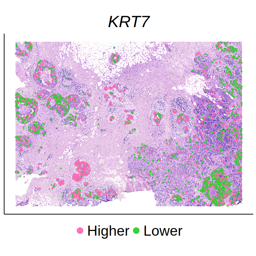
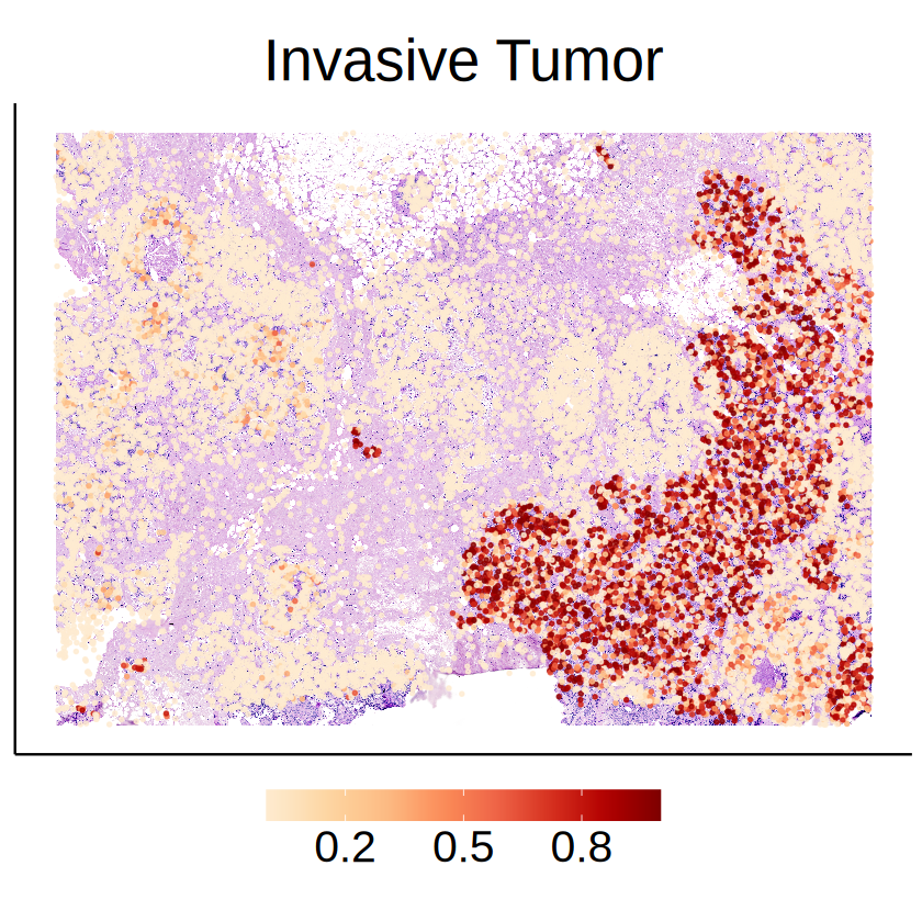
Some of cell-type-specific SVGs exhibit distinct expression patterns across different spatial domains, suggesting that these spatial variations were driven by the activities of other cells in the niche of the target cell type with high probability. For example, the expressions of CEACAM6 in DCIS 2 cells seem to be affected by surrounding Invasive Tumor cells.
[34]:
celltype <- "Invasive Tumor"
plot_df <- data.frame(
    x = mcube_object@coordinates[, 2],
    y = mcube_object@coordinates[, 1],
    prop = mcube_object@proportions[, celltype]
)
plot_df <- plot_df[plot_df$prop > 0, , drop = FALSE]

p <- ggplot(data = plot_df, aes(x = x, y = y)) +
annotation_raster(
    he_image,
    xmin = -max(mcube_object@coordinates[, 2]), xmax = 0,
    ymin = 0, ymax = max(mcube_object@coordinates[, 1])
) +
    geom_point(aes(color = prop), size = 0.5, alpha = 0.8) +
    scale_x_continuous(transform = "reverse") +
    scale_colour_gradientn(
        name = NULL,
        colors = pals::brewer.orrd(22)[3:22],
        breaks = c(0.2,0.5,0.8)) +
    guides(color = guide_colorbar(barwidth = 15)) +
    coord_fixed(ratio = 1) +
    labs(title = celltype, x = NULL, y = NULL) +
    theme_classic() +
    theme(
        text = element_text(family = "Helvetica"),
        plot.title = element_text(size = 32, hjust = 0.5),
        axis.title = element_blank(),
        axis.ticks = element_blank(),
        axis.text = element_blank(),
        legend.position = "bottom",
        legend.title = element_blank(),
        legend.text = element_text(size = 24),
    )
ggsave(
    filename = file.path(RESULT_PATH, paste0(celltype, "_proportion.png")),
    plot = p, width = 5, height = 5
)
p
[ ]: